Introduction to Customer Segmentation in Python

In the Retail sector, the various chain of hypermarkets generating an exceptionally large amount of data. This data is generated on a daily basis across the stores. This extensive database of customers transactions needs to analyze for designing profitable strategies.

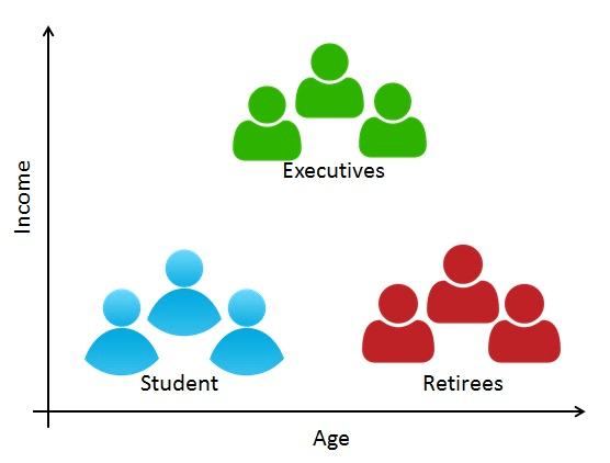
All customers have different-different kind of needs. With the increase in customer base and transaction, it is not easy to understand the requirement of each customer. Identifying potential customers can improve the marketing campaign, which ultimately increases the sales. Segmentation can play a better role in grouping those customers into various segments.

What is Customer Segmentation?

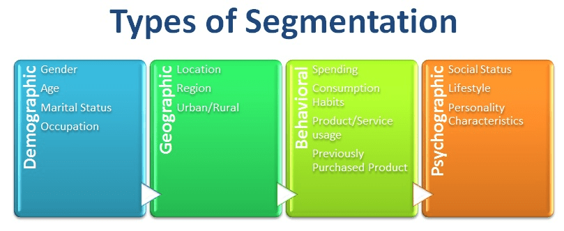
Customer segmentation is a method of dividing customers into groups or clusters on the basis of common characteristics. The market researcher can segment customers into the B2C model using various customer's demographic characteristics such as occupation, gender, age, location, and marital status. Psychographic characteristics such as social class, lifestyle and personality characteristics and behavioral characteristics such as spending, consumption habits, product/service usage, and previously purchased products. In the B2B model using various company's characteristics such as the size of the company, type of industry, and location.

Need of Customer Segmentation

• It will help in identifying the most potential customers.
• It will help managers to easily communicate with a targetted group of the audience.
• Also, help in selecting the best medium for communicating with the targetted segment.
• It improves the quality of service, loyalty, and retention.
• Improve customer relationship via better understanding needs of segments.
• It provides opportunities for upselling and cross-selling.
• It will help managers to design special offers for targetted customers, to encourage them to buy more products.
• It helps companies to stay a step ahead of competitors.
• It also helps in identifying new products that customers could be interested in.

Types of Segmentation

Customer Segmentation using RFM analysis

RFM (Recency, Frequency, Monetary) analysis is a behavior-based approach grouping customers into segments. It groups the customers on the basis of their previous purchase transactions. How recently, how often, and how much did a customer buy. RFM filters customers into various groups for the purpose of better service. It helps managers to identify potential customers to do more profitable business. There is a segment of customer who is the big spender but what if they purchased only once or how recently they purchased? Do they often purchase our product? Also, It helps managers to run an effective promotional campaign for personalized service.

• Recency (R): Who have purchased recently? Number of days since last purchase (least recency)
• Frequency (F): Who has purchased frequently? It means the total number of purchases. ( high frequency)
• Monetary Value(M): Who have high purchase amount? It means the total money customer spent (high monetary value)

Here, Each of the three variables(Recency, Frequency, and Monetary) consists of four equal groups, which creates 64 (4x4x4) different customer segments.

Steps of RFM(Recency, Frequency, Monetary):

1. Calculate the Recency, Frequency, Monetary values for each customer.
2. Add segment bin values to RFM table using quartile.
3. Sort the customer RFM score in ascending order.

1. Calculate the Recency, Frequency, Monetary values for each customer.

2. Add segment bin values to RFM table using quartile.

3. Concate all scores in single column(RFM_Score).

Identify Potential Customer Segments using RFM in Python

Importing Required Library

#import modules
import pandas as pd # for dataframes
import matplotlib.pyplot as plt # for plotting graphs
import seaborn as sns # for plotting graphs
import datetime as dt

Loading Dataset

Let's first load the required HR dataset using the pandas read CSV function. You can download the data from this link.

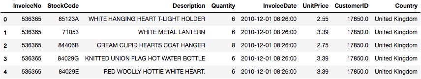
data = pd.read_excel("Online_Retail.xlsx")

data.head()

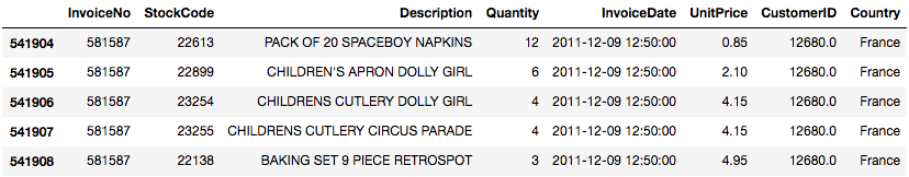
data.tail()

data.info()

<class 'pandas.core.frame.DataFrame'>
RangeIndex: 541909 entries, 0 to 541908
Data columns (total 8 columns):
InvoiceNo      541909 non-null object
StockCode      541909 non-null object
Description    540455 non-null object
Quantity       541909 non-null int64
InvoiceDate    541909 non-null datetime64[ns]
UnitPrice      541909 non-null float64
CustomerID     406829 non-null float64
Country        541909 non-null object
dtypes: datetime64[ns](1), float64(2), int64(1), object(4)
memory usage: 33.1+ MB

data= data[pd.notnull(data['CustomerID'])]

Removing Duplicates

Sometimes you get a messy dataset. You may have to deal with duplicates, which will skew your analysis. In python, pandas offer function drop_duplicates(), which drops the repeated or duplicate records.

filtered_data=data[['Country','CustomerID']].drop_duplicates()

Let's Jump into Data Insights

#Top ten country's customer
filtered_data.Country.value_counts()[:10].plot(kind='bar')

<matplotlib.axes._subplots.AxesSubplot at 0x7fd81725dfd0>

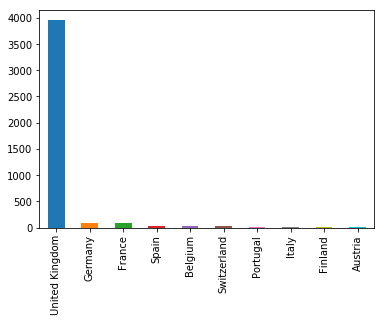
In the given dataset, you can observe most of the customers are from the "United Kingdom". So, you can filter data for United Kingdom customer.

uk_data=data[data.Country=='United Kingdom']

uk_data.info()

<class 'pandas.core.frame.DataFrame'>
Int64Index: 361878 entries, 0 to 541893
Data columns (total 8 columns):
InvoiceNo      361878 non-null object
StockCode      361878 non-null object
Description    361878 non-null object
Quantity       361878 non-null int64
InvoiceDate    361878 non-null datetime64[ns]
UnitPrice      361878 non-null float64
CustomerID     361878 non-null float64
Country        361878 non-null object
dtypes: datetime64[ns](1), float64(2), int64(1), object(4)
memory usage: 24.8+ MB

The describe() function in pandas is convenient in getting various summary statistics. This function returns the count, mean, standard deviation, minimum and maximum values and the quantiles of the data.

uk_data.describe()

Here, you can observe some of the customers have ordered in a negative quantity, which is not possible. So, you need to filter Quantity greater than zero.

uk_data = uk_data[(uk_data['Quantity']>0)]

In: # Change the name of columns
rfm.columns=['monetary','frequency','recency']

uk_data.info() 

<class 'pandas.core.frame.DataFrame'>
Int64Index: 354345 entries, 0 to 541893
Data columns (total 8 columns):
InvoiceNo      354345 non-null object
StockCode      354345 non-null object
Description    354345 non-null object
Quantity       354345 non-null int64
InvoiceDate    354345 non-null datetime64[ns]
UnitPrice      354345 non-null float64
CustomerID     354345 non-null float64
Country        354345 non-null object
dtypes: datetime64[ns](1), float64(2), int64(1), object(4)
memory usage: 24.3+ MB

Filter required Columns

Here, you can filter the necessary columns for RFM analysis. You only need her five columns CustomerID, InvoiceDate, InvoiceNo, Quantity, and UnitPrice. CustomerId will uniquely define your customers, InvoiceDate help you calculate recency of purchase, InvoiceNo helps you to count the number of time transaction performed(frequency). Quantity purchased in each transaction and UnitPrice of each unit purchased by the customer will help you to calculate the total purchased amount.

uk_data=uk_data[['CustomerID','InvoiceDate','InvoiceNo','Quantity','UnitPrice']]

uk_data['TotalPrice'] = uk_data['Quantity'] * uk_data['UnitPrice']

uk_data['InvoiceDate'].min(),uk_data['InvoiceDate'].max()

(Timestamp('2010-12-01 08:26:00'), Timestamp('2011-12-09 12:49:00'))

PRESENT = dt.datetime(2011,12,10)
uk_data['InvoiceDate'] = pd.to_datetime(uk_data['InvoiceDate'])

uk_data.head()

RFM Analysis

Here, you are going to perform following opertaions:

• For Recency, Calculate the number of days between present date and date of last purchase each customer.
• For Frequency, Calculate the number of orders for each customer.
• For Monetary, Calculate sum of purchase price for each customer.

rfm= uk_data.groupby('CustomerID').agg({'InvoiceDate': lambda date: (PRESENT - date.max()).days,
                                        'InvoiceNo': lambda num: len(num),
                                        'TotalPrice': lambda price: price.sum()})

rfm.columns

Index(['InvoiceDate', 'TotalPrice', 'InvoiceNo'], dtype='object')

# Change the name of columns 
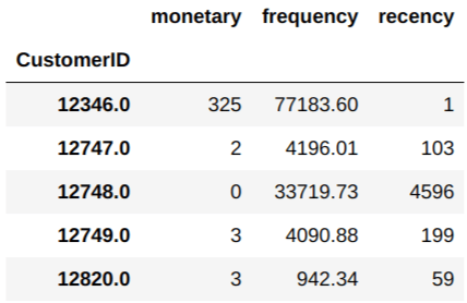
rfm.columns=['recency', 'monetary', 'frequency'] 

rfm['recency'] = rfm['recency'].astype(int)

rfm.head()

Computing Quantile of RFM values

Customers with the lowest recency, highest frequency and monetary amounts considered as top customers.

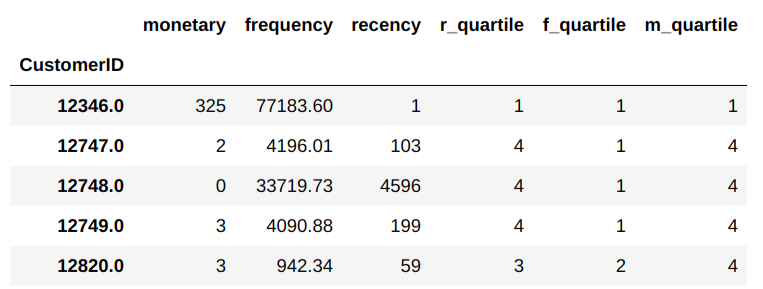
qcut() is Quantile-based discretization function. qcut bins the data based on sample quantiles. For example, 1000 values for 4 quantiles would produce a categorical object indicating quantile membership for each customer.

rfm['r_quartile'] = pd.qcut(rfm['recency'], 4, ['1','2','3','4'])
rfm['f_quartile'] = pd.qcut(rfm['frequency'], 4, ['4','3','2','1'])
rfm['m_quartile'] = pd.qcut(rfm['monetary'], 4, ['4','3','2','1'])

rfm.head()

RFM Result Interpretation

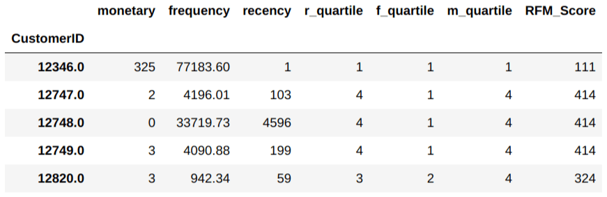
Combine all three quartiles(r_quartile,f_quartile,m_quartile) in a single column, this rank will help you to segment the customers well group.

rfm['RFM_Score'] = rfm.r_quartile.astype(str)+ rfm.f_quartile.astype(str) + rfm.m_quartile.astype(str)
rfm.head()

# Filter out Top/Best cusotmers
rfm[rfm['RFM_Score']=='111'].sort_values('monetary', ascending=False).head()

Conclusion

Congratulations, you have made it to the end of this tutorial!

In this tutorial, you covered a lot of details about Customer Segmentation. You have learned what the customer segmentation is, Need of Customer Segmentation, Types of Segmentation, RFM analysis, Implementation of RFM from scratch in python. Also, you covered some basic concepts of pandas such as handling duplicates, groupby, and qcut() for bins based on sample quantiles.

Hopefully, you can now utilize topic modeling to analyze your own datasets. Thanks for reading this tutorial!

If you want to learn more about Python, take DataCamp's free Intro to Python for Data Science course.