An Introduction to Q-Learning: A Tutorial For Beginners

Reinforcement learning (RL) is the part of the machine learning ecosystem where the agent learns by interacting with the environment to obtain the optimal strategy for achieving the goals. It is quite different from supervised machine learning algorithms, where we need to ingest and process that data. Reinforcement learning does not require data. Instead, it learns from the environment and reward system to make better decisions.

For example, in the Mario video game, if a character takes a random action (e.g. moving left), based on that action, it may receive a reward. After taking the action, the agent (Mario) is in a new state, and the process repeats until the game character reaches the end of the stage or dies. 

This episode will repeat multiple times until Mario learns to navigate the environment by maximizing the rewards. 

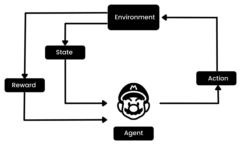
Image by Author

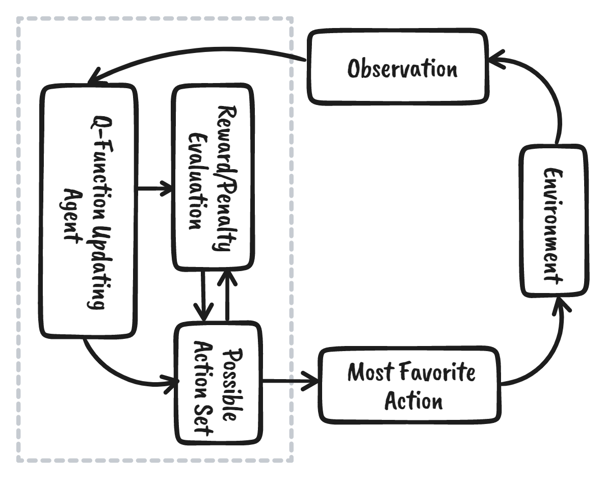
We can break down reinforcement learning into five simple steps:

1. The agent is at state zero in an environment.
2. It will take an action based on a specific strategy.
3. It will receive a reward or punishment based on that action.
4. By learning from previous moves and optimizing the strategy. 
5. The process will repeat until an optimal strategy is found. 

Learn more by reading our tutorial, an Introduction to Reinforcement Learning. You’ll explore more about how reinforcement learning works with code examples. 

In this tutorial, we will learn about Q-learning and understand why we need Deep Q-learning. Moreover, we will learn to create and train Q-learning algorithms from scratch using Numpy and OpenAI Gym.

Note: If you are new to machine learning, we recommend you take our Machine Learning Scientist with Python career track to better understand Reinforcement learning and Q-Learning. 

What is Q-Learning?

Q-learning is a model-free, value-based, off-policy algorithm that will find the best series of actions based on the agent's current state. The “Q” stands for quality. Quality represents how valuable the action is in maximizing future rewards.  

The model-based algorithms use transition and reward functions to estimate the optimal policy and create the model. In contrast, model-free algorithms learn the consequences of their actions through the experience without transition and reward function. 

The value-based method trains the value function to learn which state is more valuable and take action. On the other hand, policy-based methods train the policy directly to learn which action to take in a given state.

In the off-policy, the algorithm evaluates and updates a policy that differs from the policy used to take an action. Conversely, the on-policy algorithm evaluates and improves the same policy used to take an action.  

Key Terminologies in Q-learning

Before we jump into how Q-learning works, we need to learn a few useful terminologies to understand Q-learning's fundamentals. 

• States(s): the current position of the agent in the environment. 
• Action(a): a step taken by the agent in a particular state. 
• Rewards: for every action, the agent receives a reward and penalty. 
• Episodes: the end of the stage, where agents can’t take new action. It happens when the agent has achieved the goal or failed. 
• Q(S_t+1, a): expected optimal Q-value of doing the action in a particular state. 
• Q(S_t, A_t): it is the current estimation of Q(S_t+1, a).
• Q-Table: the agent maintains the Q-table of sets of states and actions.
• Temporal Differences(TD): used to estimate the expected value of Q(S_t+1, a) by using the current state and action and previous state and action. 

How Does Q-Learning Work?

We will learn in detail how Q-learning works by using the example of a frozen lake. In this environment, the agent must cross the frozen lake from the start to the goal, without falling into the holes. The best strategy is to reach goals by taking the shortest path. 

Gif by Author

Q-Table

The agent will use a Q-table to take the best possible action based on the expected reward for each state in the environment. In simple words, a Q-table is a data structure of sets of actions and states, and we use the Q-learning algorithm to update the values in the table. 

Q-Function

The Q-function uses the Bellman equation and takes state(s) and action(a) as input. The equation simplifies the state values and state-action value calculation.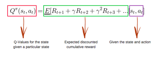 

Image from freecodecamp.org

Q-learning algorithm

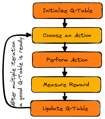
Image by Author

Initialize Q-Table

We will first initialize the Q-table. We will build the table with columns based on the number of actions and rows based on the number of states.

In our example, the character can move up, down, left, and right. We have four possible actions and four states(start, Idle, wrong path, and end). You can also consider the wrong path for falling into the hole. We will initialize the Q-Table with values at 0. 

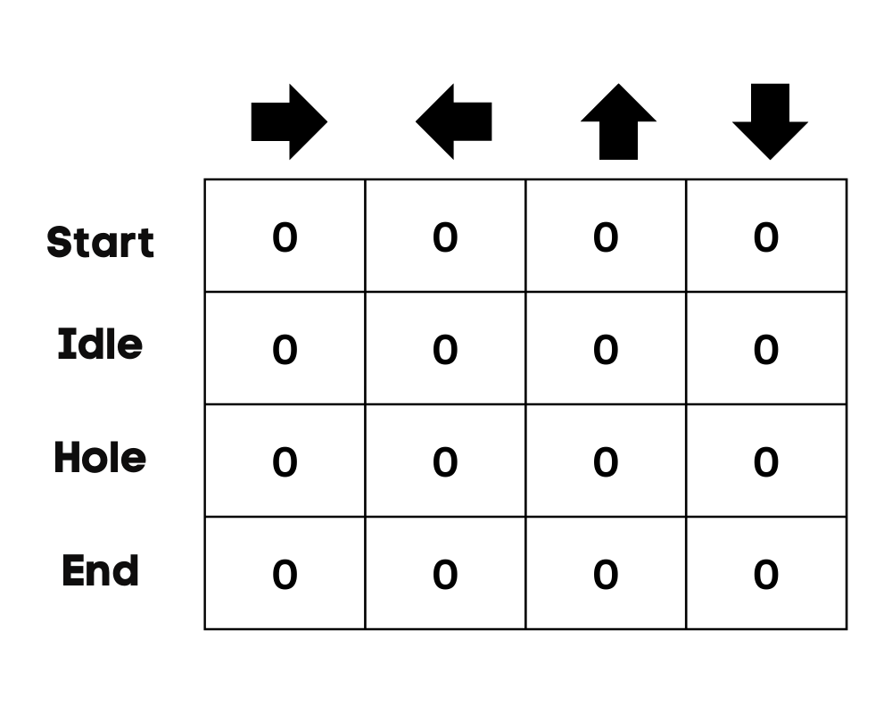
Image by Author

Choose an Action

The second step is quite simple. At the start, the agent will choose to take the random action(down or right), and on the second run, it will use an updated Q-Table to select the action. 

Perform an Action

Choosing an action and performing the action will repeat multiple times until the training loop stops. The first action and state are selected using the Q-Table. In our case, all values of the Q-Table are zero. 

Then, the agent will move down and update the Q-Table using the Bellman equation. With every move, we will be updating values in the Q-Table and also using it for determining the best course of action. 

Initially, the agent is in exploration mode and chooses a random action to explore the environment. The Epsilon Greedy Strategy is a simple method to balance exploration and exploitation. The epsilon stands for the probability of choosing to explore and exploits when there are smaller chances of exploring. 

At the start, the epsilon rate is higher, meaning the agent is in exploration mode. While exploring the environment, the epsilon decreases, and agents start to exploit the environment. During exploration, with every iteration, the agent becomes more confident in estimating Q-values

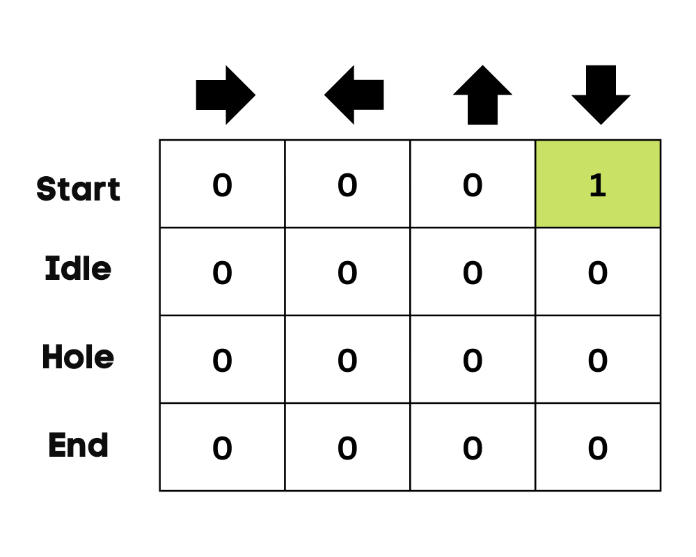
Image by Author

In the frozen lake example, the agent is unaware of the environment, so it takes random action (move down) to start. As we can see in the above image, the Q-Table is updated using the Bellman equation.

Measuring the Rewards

After taking the action, we will measure the outcome and the reward. 

• The reward for reaching the goal is +1
• The reward for taking the wrong path (falling into the hole) is 0
• The reward for Idle or moving on the frozen lake is also 0. 

Update Q-Table

We will update the function Q(S_t, A_t) using the equation. It uses the previous episode’s estimated Q-values, learning rate, and Temporal Differences error. Temporal Differences error is calculated using Immediate reward, the discounted maximum expected future reward, and the former estimation Q-value. 

The process is repeated multiple times until the Q-Table is updated and the Q-value function is maximized. 

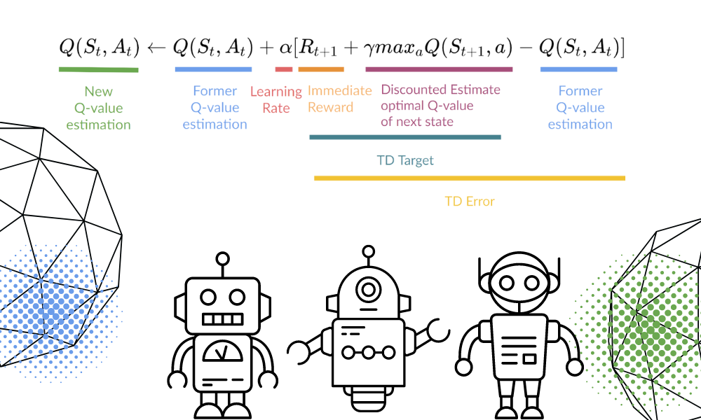
Image by Author | Equation Visuals from Thomas Simonini

At the start, the agent is exploring the environment to update the Q-table. And when the Q-Table is ready, the agent will start exploiting and start taking better decisions.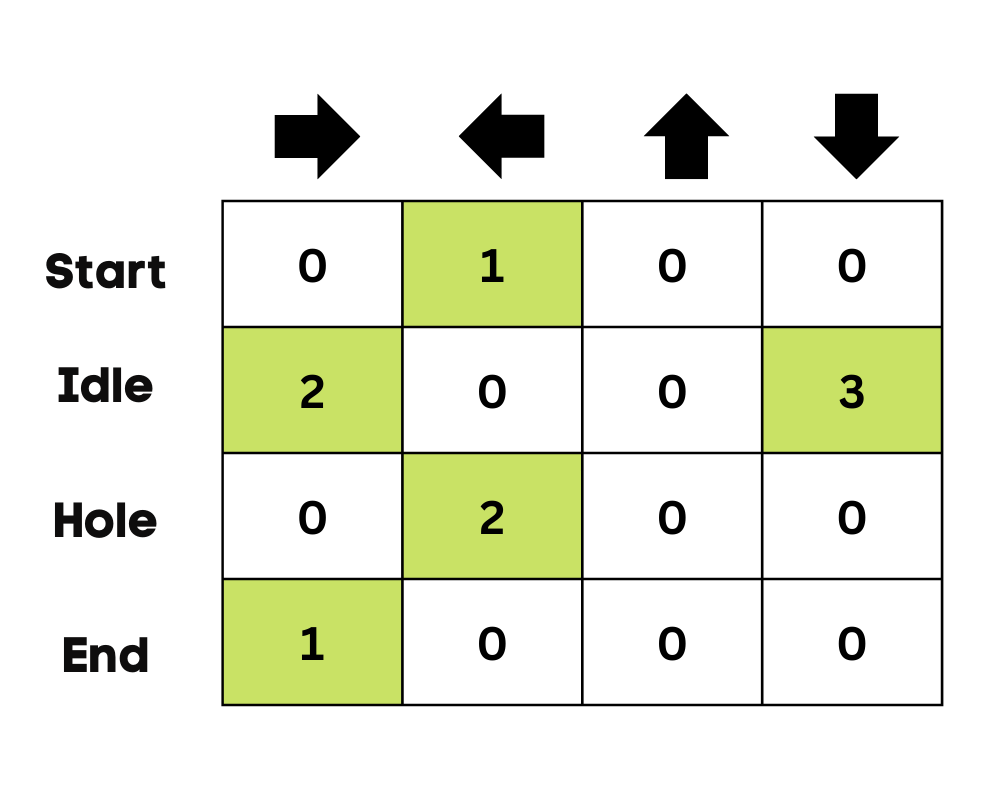 

Image by Author

In the case of a frozen lake, the agent will learn to take the shortest path to reach the goal and avoid jumping into the holes. 

Q-Learning Python Tutorial 

In this section, we will build our Q-learning model from scratch using the Gym environment, Pygame, and Numpy. The Python tutorial is a modified version of the Notebook by Thomas Simonini. It includes initializing the environment and Q-Table, defining greedy policy, setting hyperparameters, creating and running the training loop and evaluation, and visualizing the results.   

If you are facing issues creating and running your training loop, you can check the code source with the output.   

Setting Up

Setup a Virtual Display

We will first install all the dependencies to generate a replay video(Gif). We will need a virtual screen (pyvirtualdisplay) to render the environment and record the frames. 

Note: by using `%%capture` we are suppressing the output of the Jupyter cell. 

%%capture
!pip install pyglet==1.5.1
!apt install python-opengl
!apt install ffmpeg
!apt install xvfb
!pip3 install pyvirtualdisplay

# Virtual display
from pyvirtualdisplay import Display

virtual_display = Display(visible=0, size=(1400, 900))
virtual_display.start()

Install dependencies

We will now install dependencies that will help us create, run, and evaluate the training loop. 

• gym: Used to initialize the FrozenLake-v1 environment.
• pygame: Used for the FrozenLake-v1 UI.
• numPy: Used for creating and handling the Q-table.

%%capture
!pip install gym==0.24
!pip install pygame
!pip install numpy

!pip install imageio imageio_ffmpeg

Import the packages

We will now import the required libraries. 

• Imageio is used for creating the animation. 
• tqdm is used for progress bars. 

import numpy as np
import gym
import random
import imageio
from tqdm.notebook import trange

Frozen Lake Gym Environment 

We are going to create a non-slippery 4x4 environment using the Frozen Lake gym library. 

• There are two grid versions, “4x4” and “8x8”.
• If the `is_slippery=True`, the agent may not move in the intended direction due to the slippery nature of the frozen lake. 

After initializing the environment, we will do an environmental analysis. 

env = gym.make("FrozenLake-v1",map_name="4x4",is_slippery=False)

print("Observation Space", env.observation_space)
print("Sample observation", env.observation_space.sample()) # display a random observation

There are 16 unique spaces in the environment displayed at random positions. 

Observation Space Discrete(16)
Sample observation 15

Let’s discover the number of actions and display the random action. 

The action space:

• 0: move left
• 1: move down
• 2: move right
• 3: move up

Reward function:

• Reaching the goal: +1
• Falling into the hole: 0
• Staying on the frozen lake: 0

print("Action Space Shape", env.action_space.n)
print("Action Space Sample", env.action_space.sample())

Action Space Shape 4
Action Space Sample 1

Create and Initialize the Q-table

The Q-Table has columns as actions, and rows as states. We can use OpenAI Gym to find action space and state space. We will then use this information to create the Q-Table. 

state_space = env.observation_space.n
print("There are ", state_space, " possible states")

action_space = env.action_space.n
print("There are ", action_space, " possible actions")

There are  16  possible states
There are  4  possible actions

For initializing the Q-Table, we will create a Numpy array of state_space and actions space. We will create a 16 X 4 array. 

def initialize_q_table(state_space, action_space):
  Qtable = np.zeros((state_space, action_space))
  return Qtable

Qtable_frozenlake = initialize_q_table(state_space, action_space)

Epsilon-greedy policy

In the previous section, we have learned about the epsilon greedy strategy that handles exploration and exploitation tradeoffs. With a Probability of 1 - ɛ, we do exploitation, and with the probability ɛ, we do exploration. 

In the epsilon_greedy_policy we will:

1. Generate the random number between 0 to 1.
2. If the random number is greater than epsilon, we will do exploitation. It means that the agent will take the action with the highest value given a state.
3. Else, we will do exploration (Taking random action). 

def epsilon_greedy_policy(Qtable, state, epsilon):
  random_int = random.uniform(0,1)
  if random_int > epsilon:
    action = np.argmax(Qtable[state])
  else:
    action = env.action_space.sample()
  return action

Define the greedy policy

As we now know that Q-learning is an off-policy algorithm which means that the policy of taking action and updating function is different. 

In this example, the Epsilon Greedy policy is acting policy, and the Greedy policy is updating policy. 

The Greedy policy will also be the final policy when the agent is trained. It is used to select the highest state and action value from the Q-Table.

def greedy_policy(Qtable, state):
  action = np.argmax(Qtable[state])
  return action

Model hyperparameters

These hyperparameters are used in the training loop, and fine-tuning them will give you better results. 

The Agent needs to explore enough state space to learn good value approximation; we need to have progressive decay of epsilon. If the decay rate is high, the agent might get stuck as it has not explored enough state space.

• There are 10,000 training and 100 evaluation episodes.
• The learning rate is 0.7.
• We are using "FrozenLake-v1" as an environment with 99 maximum steps per episode.
• The gamma (discount rate) is 0.95.
• eval_seed: evaluation seed for the environment.
• The exploration epsilon probability at the start is 1.0, and the minimum probability will be 0.05.
• The exponential decay rate for epsilon probability is 0.0005.

# Training parameters
n_training_episodes = 10000
learning_rate = 0.7        

# Evaluation parameters
n_eval_episodes = 100      

# Environment parameters
env_id = "FrozenLake-v1"   
max_steps = 99             
gamma = 0.95               
eval_seed = []             

# Exploration parameters
max_epsilon = 1.0           
min_epsilon = 0.05           
decay_rate = 0.0005           

Model Training 

In the training loop, we will:

1. Create a loop for training episodes.
2. We will first reduce epsilon. As we need less and less exploration and more exploitation with every episode. 
3. Reset the environment.
4. Create a nested loop for the maximum steps.
5. Choose the action using the epsilon greedy policy. 
6. Take action (A_t) and observe the expected reward(R_t+1) and state(S_t+1).
7. Take the action (a) and observe the outcome state(s') and reward (r).
8. Update the Q-function using the formula. 
9. If `done= True`, finish the episode and break the loop.
10. Finally, change the current state to a new state. 
11. After completing all of the training episodes, the function will return the updated Q-Table. 

def train(n_training_episodes, min_epsilon, max_epsilon, decay_rate, env, max_steps, Qtable):
  for episode in trange(n_training_episodes):
 
    epsilon = min_epsilon + (max_epsilon - min_epsilon)*np.exp(-decay_rate*episode)
    # Reset the environment
    state = env.reset()
    step = 0
    done = False

    # repeat
    for step in range(max_steps):
   
      action = epsilon_greedy_policy(Qtable, state, epsilon)

   
      new_state, reward, done, info = env.step(action)

   
      Qtable[state][action] = Qtable[state][action] + learning_rate * (reward + gamma * np.max(Qtable[new_state]) - Qtable[state][action])

      # If done, finish the episode
      if done:
        break
     
      # Our state is the new state
      state = new_state
  return Qtable

It took us 3 seconds to finish 10,000 training episodes. 

Qtable_frozenlake = train(n_training_episodes, min_epsilon, max_epsilon, decay_rate, env, max_steps, Qtable_frozenlake)

As we can see, the trained Q-Table has values, and the agent will now use these values to navigate the environment and achieve the goal.  

Qtable_frozenlake

array([[0.73509189, 0.77378094, 0.77378094, 0.73509189],
      [0.73509189, 0.        , 0.81450625, 0.77378094],
      [0.77378094, 0.857375  , 0.77378094, 0.81450625],
      [0.81450625, 0.        , 0.77378094, 0.77378094],
      [0.77378094, 0.81450625, 0.        , 0.73509189],
      [0.        , 0.        , 0.        , 0.        ],
      [0.        , 0.9025    , 0.        , 0.81450625],
      [0.        , 0.        , 0.        , 0.        ],
      [0.81450625, 0.        , 0.857375  , 0.77378094],
      [0.81450625, 0.9025    , 0.9025    , 0.        ],
      [0.857375  , 0.95      , 0.        , 0.857375  ],
      [0.        , 0.        , 0.        , 0.        ],
      [0.        , 0.        , 0.        , 0.        ],
      [0.        , 0.9025    , 0.95      , 0.857375  ],
      [0.9025    , 0.95      , 1.        , 0.9025    ],
      [0.        , 0.        , 0.        , 0.        ]])

Evaluation

The evaluate_agent runs for `n_eval_episodes` episodes and returns the mean and standard deviation of the reward. 

1. In the loop, we will first check if there is an evaluation seed. If not, then we will reset the environment without seed. 
2. The nested loop will run to max_steps.
3. The agent will take the action that has the maximum expected future reward in a given state using Q-Table. 
4. Calculate the reward.
5. Change the state.
6. If done (agent falls into the hole or goal has been achieved), break the loop.
7. Append the results.
8. In the end, we will use these results to calculate the mean and standard deviation. 

def evaluate_agent(env, max_steps, n_eval_episodes, Q, seed):

  episode_rewards = []
  for episode in range(n_eval_episodes):
    if seed:
      state = env.reset(seed=seed[episode])
    else:
      state = env.reset()
    step = 0
    done = False
    total_rewards_ep = 0
   
    for step in range(max_steps):
      # Take the action (index) that have the maximum reward
      action = np.argmax(Q[state][:])
      new_state, reward, done, info = env.step(action)
      total_rewards_ep += reward
       
      if done:
        break
      state = new_state
    episode_rewards.append(total_rewards_ep)
  mean_reward = np.mean(episode_rewards)
  std_reward = np.std(episode_rewards)

  return mean_reward, std_reward

As you can see, we got the perfect score with zero standard deviation. It means that our agent has reached the goal in all 100 episodes. 

# Evaluate our Agent
mean_reward, std_reward = evaluate_agent(env, max_steps, n_eval_episodes, Qtable_frozenlake, eval_seed)
print(f"Mean_reward={mean_reward:.2f} +/- {std_reward:.2f}")

Mean_reward=1.00 +/- 0.00

Visualizing the result

Till now, we have been playing with numbers, and to give the demo, we need to create an animated Gif of the agent from the start till it reaches the goal. 

1. We will first create the state by resetting the environment with a random integer 0-500. 
2. Render the environment using rdb_array to create an image array. 
3. Then append the `img` to the `images` array. 
4. In the loop, we will take the step using the Q-Table and render the image for every step. 
5. In the end, we will use this array and imageio to create a Gif of one frame per second. 

def record_video(env, Qtable, out_directory, fps=1):
  images = [] 
  done = False
  state = env.reset(seed=random.randint(0,500))
  img = env.render(mode='rgb_array')
  images.append(img)
  while not done:
    # Take the action (index) that have the maximum expected future reward given that state
    action = np.argmax(Qtable[state][:])
    state, reward, done, info = env.step(action) # We directly put next_state = state for recording logic
    img = env.render(mode='rgb_array')
    images.append(img)
  imageio.mimsave(out_directory, [np.array(img) for i, img in enumerate(images)], fps=fps)

If you are in a Jupyter notebook, you can display the Gif using the `IPython.display` Image function. 

video_path="/content/replay.gif"
video_fps=1
record_video(env, Qtable_frozenlake, video_path, video_fps)

from IPython.display import Image
Image('./replay.gif')

You can now share these results with your colleagues and class fellows or post them on social media.