Recommendation System for Streaming Platforms Tutorial

Due to the new culture of Binge-watching TV Shows and Movies, users are consuming content at a fast pace with available services like Netflix, Prime Video, Hulu, and Disney+. Some of these new platforms, such as Hulu and YouTube TV, also offer live streaming of events like Sports, live concerts/tours, and news channels. Live streaming is still not adopted by some of the streaming platforms, such as Netflix.

Streaming platforms provide more flexibility to users to watch their favorite TV shows and movies, at any time, on any device. These services can attract more young and modern consumers because of its wide variety of TV and movie content. It allows them to watch any missed program as their availability. In this tutorial, you will analyze movie data of streaming platforms Netflix, Prime Video, Hulu, and Disney+ and try to understand their viewers.

Understanding the Dataset

This data consisted of only movies available on streaming platforms such as Netflix, Prime Video, Hulu, and Disney+. You can download it from Kaggle here.

Let's describe data attributes in detail:

• ID: It is a unique ID for each record.
• Title: It is the name of the movie
• Year: Release year of the movie.
• Age: it is the target age group
• IMDb: IMDB rating of movies.
• Rotten Tomatoes: Rotten Tomatoes %
• Netflix: whether the movie is found on Netflix
• Hulu: whether the movie is found on Hulu
• Prime Video: whether the movie is found on Prime Video
• Disney+: whether the movie is found on Disney+
• Type: Movie or TV show
• Directors: Name of the director
• Genres: Type of genre
• Country: Country of origin
• Language: Language of origin
• Runtime: Duration of the movie

Let's import the necessary modules and load the dataset:

 # Import required libraries
import numpy as np
import pandas as pd
import matplotlib.pyplot as plt
import seaborn as sns
from sklearn.feature_extraction.text import TfidfVectorizer    
from nltk.tokenize import RegexpTokenizer
import numpy as np
from sklearn import preprocessing
from scipy.sparse import hstack
import pandas_profiling

# Load dataset
df = pd.read_csv("tvshow.csv")
df=df.iloc[:,1:] # removing in unnamed index column

df.head()

# Show initial information about the dataset
df.info()

<class 'pandas.core.frame.DataFrame'>
RangeIndex: 16744 entries, 0 to 16743
Data columns (total 16 columns):
 #   Column           Non-Null Count  Dtype  
---  ------           --------------  -----  
 0   ID               16744 non-null  object
 1   Title            16744 non-null  object
 2   Year             16744 non-null  int64  
 3   Age              7354 non-null   object
 4   IMDb             16173 non-null  float64
 5   Rotten Tomatoes  5158 non-null   object
 6   Netflix          16744 non-null  int64  
 7   Hulu             16744 non-null  int64  
 8   Prime Video      16744 non-null  int64  
 9   Disney+          16744 non-null  int64  
 10  Type             16744 non-null  int64  
 11  Directors        16018 non-null  object
 12  Genres           16469 non-null  object
 13  Country          16309 non-null  object
 14  Language         16145 non-null  object
 15  Runtime          16152 non-null  float64
dtypes: float64(2), int64(6), object(8)
memory usage: 2.0+ MB

df.Type.unique()

array([0])

Working with Missing Values

In this section, You will work with missing values using the isnull() function. Let's see an example below:

 #Finding Missing values in all columns
miss = pd.DataFrame(df.isnull().sum())
miss = miss.rename(columns={0:"miss_count"})
miss["miss_%"] = (miss.miss_count/len(df.ID))*100
miss

You can see that the variables Age and Rotten tomatoes have more than 50 % missing values, which is alarming.

Now, we will handle the missing values in the following steps:

• Drop columns which has more than 50% missing values
• Drop NA from IMDb, Directors, Genres, Country, Language, and Runtime column
• Reset index
• Convert year column into object

# Dropping values with missing % more than 50%
df.drop(['Rotten Tomatoes', 'Age'], axis = 1, inplace=True)
# Dropping Na's from the following columns
df.dropna(subset=['IMDb','Directors', 'Genres', 'Country', 'Language', 'Runtime'],inplace=True)
df.reset_index(inplace=True,drop=True)
# Converting into object type
df.Year = df.Year.astype("object")

df.info()

<class 'pandas.core.frame.DataFrame'>
RangeIndex: 15233 entries, 0 to 15232
Data columns (total 14 columns):
 #   Column       Non-Null Count  Dtype  
---  ------       --------------  -----  
 0   ID           15233 non-null  object
 1   Title        15233 non-null  object
 2   Year         15233 non-null  object
 3   IMDb         15233 non-null  float64
 4   Netflix      15233 non-null  int64  
 5   Hulu         15233 non-null  int64  
 6   Prime Video  15233 non-null  int64  
 7   Disney+      15233 non-null  int64  
 8   Type         15233 non-null  int64  
 9   Directors    15233 non-null  object
 10  Genres       15233 non-null  object
 11  Country      15233 non-null  object
 12  Language     15233 non-null  object
 13  Runtime      15233 non-null  float64
dtypes: float64(2), int64(5), object(7)
memory usage: 1.6+ MB

Distribution Plots

You can check the distribution of the Year column using the distplot() function of seaborn. Let's plot the Movie Year distribution plot.

#checking Distribution of years
plt.figure(figsize=(20,5))
sns.distplot(df['Year'])
plt.show()

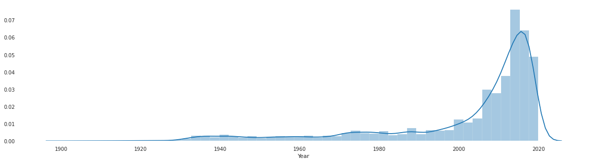
The chart is showing the distribution of movies origin year. You can interpret that most of the movies were made between the year 2000 to 2020. Let's plot the IMDB rating distribution plot.

# Distribution of IMDb Rating
plt.figure(figsize=(20,5))
sns.distplot(df['IMDb'])
plt.show()

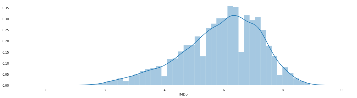
The above distribution plot is slightly skewed. You can interpret that the mean IMDB of most movies is 6.5.

Let's plot the Movie Runtime distribution plot.

# Distribution of runtime
sns.distplot(df['Runtime'])
plt.show()

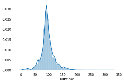
From the above chart, you can interpret that the movie's average runtime lies between 80 to 120 mins.

Distribution of Movies on each Streaming Platform

In this section, you will see Streaming Platform wise movie distribution. First, you need to create an m_cnt() function that counts movies for a given streaming platform. After that, you can plot using Pie charts and understand the shares of streaming platforms.

# A function to calculate the movies in different Streaming platforms
def m_cnt(plat, count=False):
    if count==False:
        print('Platform {} Count: {}'. format(plat, df[plat].sum()))
    else:
        return df[plat].sum()

# Let's see count of movies/shows of each streaming platform
m_cnt('Netflix')
m_cnt('Hulu')
m_cnt('Prime Video')
m_cnt('Disney+')

Platform Netflix Count: 3152
Platform Hulu Count: 848
Platform Prime Video Count: 11289
Platform Disney+ Count: 542

# Movies on each platform
lab = 'Prime Video','Netflix', 'Hulu', 'Disney'
s = [m_cnt('Prime Video', count=True),
     m_cnt('Netflix', count=True),
     m_cnt('Hulu', count=True),
     m_cnt('Disney+', count=True)]

explode = (0.1, 0.1, 0.1, 0.1)

#plotting
fig1, ax1 = plt.subplots()
ax1.pie(s,
       labels = lab,
       autopct = '%1.1f%%',
       explode = explode,
       shadow = True,
       startangle = 100)

ax1.axis = ('equal')
plt.show()

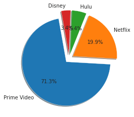
From the above plot, you can say that Prime Videos is hosting the maximum number of titles with 71% share and Netflix hosting 20% of titles. Disney+ and Hulu are hosting the lowest titles, 5.4%, and 3.4%, respectively.

Movie Distribution According to Genre

In this section, you will see genre-wise movie distribution. First, you need to prepare your data. You need to handle multiple genres given in a single cell of dataframe. For that, you can use split(), apply(), and stack() functions. split() function splits the multiple values with a comma and creates a list. apply(pd.Series,1) to create multiple columns for each genre and stack() function stack them into a single column.

After these three operations, a new Genres column will join with the existing dataframe, and you are ready to plot. You can show the top 10 genres with their movie count using value_counts() function and use plot() function of the pandas library.

 ##split the genres by ',' & then stack it one after the other for easy analysis.
g = df['Genres'].str.split(',').apply(pd.Series, 1).stack()
g.index = g.index.droplevel(-1)
# Assign name to column
g.name = 'Genres'
# delete column
del df['Genres']
# join new column with the existing dataframe
df_genres = df.join(g)

# Count of movies according to genre
plt.figure(figsize=(15,5))
sns.countplot(x='Genres', data=df_genres)
plt.xticks(rotation=90)
plt.show()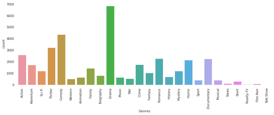

From the above plot, you can say that most of the movies have a common genre as Drama and Comedy.

Movie Distribution According to Country

In this section, you will see the country-wise movie distribution. First, you need to prepare your data. You need to handle multiple countries given in a single cell of dataframe. For that, you can use split(), apply(), and stack() functions. The split() function splits the multiple values with a comma and creates a list. apply(pd.Series,1) to create multiple columns for each country and stack() function stack them into a single column.

After these three operations, a new Country column will join with the existing dataframe and you are ready to plot. You can show the top 10 countries with their movie count using value_counts() function and use the pandas library's plot() function.

 # Split the Country by ',' & then stack it one after the other for easy analysis.
c = df['Country'].str.split(',').apply(pd.Series, 1).stack()
c.index = c.index.droplevel(-1)
# Assign name to column
c.name = 'Country'
# delete column
del df['Country']
# join new column with the existing dataframe
df_country = df.join(c)

# plotting top 10 country and movie count
df_country['Country'].value_counts()[:10].plot(kind='bar',figsize=(15,5))
plt.show()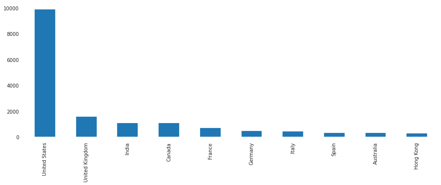

The above graph shows that the majority of the movies were made in the United States.

Movie Distribution According to Language

In this section, you will see language-wise movie distribution. First, you need to prepare your data. You need to handle multiple languages given in a single cell of the dataframe. For that, you can use split(), apply(), and stack() functions. split() function spits the multiple values with a comma and creates a list. apply(pd.Series,1) to create multiple columns for each language and stack() function stack them into a single column.

After these three operations, a new Language column will join with the existing dataframe, and you are ready to plot. You can show the top 10 languages with their movie count using value_counts() function and use the plot() function of the pandas library.

 # perform stacking operation on language column
l = df['Language'].str.split(',').apply(pd.Series,1).stack()
l.index = l.index.droplevel(-1)
# Assign name to column
l.name = 'Language'
# delete column
del df['Language']
# join new column with the existing dataframe
df_language = df.join(l)

# plotting top 10 Language and movie count
df_language['Language'].value_counts()[:10].plot(kind='bar',figsize=(15,3))
plt.show()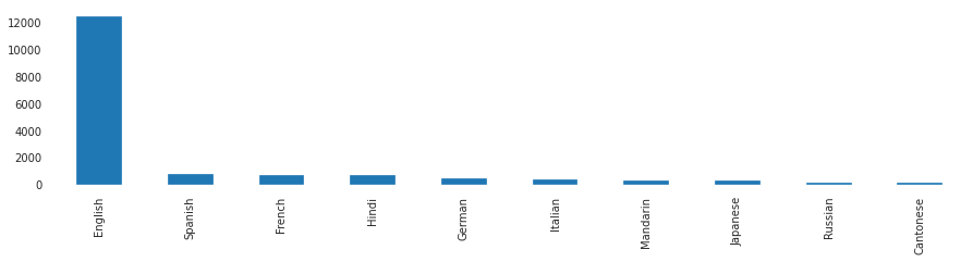

From the above plot, you can conclude that the majority of movies were in the English language.

IMDB rating Distribution According on each Platform

In this section, you will plot platform-wise IMDB rating distribution. For getting these results, you need to apply the melt() function and plot FacetGrid plot. melt() function converts a wide dataframe to a long dataframe. Let's see example below:

 # melting platform columns to create visualization
df2 = pd.melt(df, id_vars=["ID","Title","Year","IMDb","Type","Runtime"], var_name="platform")
df2 = df2[df2.value==1]
df2.drop(columns=["value"],axis=1,inplace=True)

# Distribution of IMDB rating in different platform
g = sns.FacetGrid(df2, col = "platform")
g.map(plt.hist, "IMDb")
plt.show()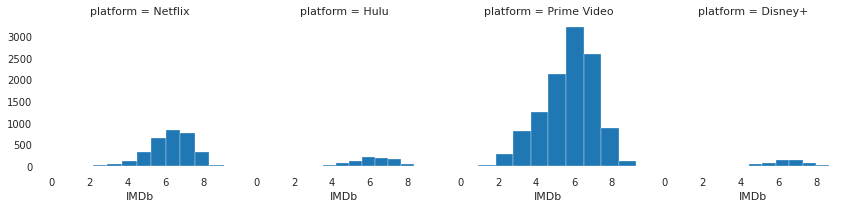

The above plot shows the average IMDB rating distribution on each platform.

Runtime Per Platform Along with Age Group

In the "Working With Missing Values Section", I have dropped the Age column. For getting results of Runtime Per Platform Along with Age Group. I need to load the data again and apply the melt() function.

# Load dataset
df = pd.read_csv("tvshow.csv")
df=df.iloc[:,1:]
df.ID = df.ID.astype("object")

# melting platform columns to create visualization
df2 = pd.melt(df, id_vars=["ID","Title","Year","Age","IMDb","Rotten Tomatoes","Type","Runtime"], var_name="platform")
df2 = df2[df2.value==1]
df2.drop(columns=["value"],axis=1,inplace=True)

After loading the dataset again and performing melting, its time to generate a plot for runtime vs. streaming platform for different age groups.

# Total of runtime in different platform
ax = sns.barplot(x="platform", y="Runtime",hue="Age", estimator=sum, data=df2)

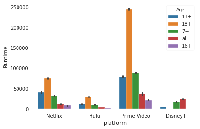
The above plot shows that the total runtime on Prime Videos by 18+ age group users is way higher than compared to any other platform. You can interpret that the Prime Videos most of the content is focused on the 18+ Age group.

Building a Recommender System

In the past few years, with the leap of YouTube, Walmart, Netflix, and many other such web-based services, recommender systems have created tremendous impact in the industry. From suggesting products/services to increasing companies value by online Ads-based monetization and matching the user's relevance and preference to make them buy. Recommender systems are irreplaceable in our daily web quests.

Generally, these are Math based frameworks focusing on suggesting products/services to end-users that are relevant to their needs and wants. For example, movies to watch, articles to read, products to buy, music to listen to, or anything depending on the domain. There are majorly three methods to build a Recommender Systems:

1. Content-Based Methods: Define a model for users or items it interacted with based on items feature set recommend other similar items to the users.
2. Collaborative Filtering Methods: Define a model for users and items interaction similarity score or User and User similarity score used for item recommendation.
3. Hybrid Methods: Use both content and collaborative methods to achieve a better result.

Let's first preprocess the dataset for the recommender system. First, you check the missing values:

# Reading Data Again
df = pd.read_csv("tvshow.csv")
df=df.iloc[:,1:]

#Finding Missing values in all columns
miss = pd.DataFrame(df.isnull().sum())
miss = miss.rename(columns={0:"miss_count"})
miss["miss_%"] = (miss.miss_count/len(df.ID))*100
miss

#Dropping values with missing % more than 50%
df.drop(['Rotten Tomatoes', 'Age'], axis = 1, inplace=True)
# Dropping Na's from the following columns
df.dropna(subset=['IMDb','Directors', 'Genres', 'Country', 'Language', 'Runtime'],inplace=True)
df.reset_index(inplace=True,drop=True)
# converting into object type
df.ID = df.ID.astype("object")
df.Year = df.Year.astype("object")

You will build two recommender system based on cosine similarity.

1. Using only the numerical variable
2. Using both numerical and categorical variable

Using only Numerical column

Step 1: Select the numerical variable

ndf = df.select_dtypes(include=['float64',"int64"])

Step 2: Scaling the numerical variable using a min-max scaler to reduce model complexity and training time

#importing minmax scaler
from sklearn import preprocessing

# Create MinMaxScaler Object
scaler = preprocessing.MinMaxScaler(feature_range=(0, 1))

# Create dataframe after transformation
ndfmx = pd.DataFrame((scaler.fit_transform(ndf)))

# assign column names
ndfmx.columns=ndf.columns

# Show initial 5 records
ndfmx.head()

Step 3: Compute similarity score using cosine similarity

Now, you will compute the similarity score using cosine similarity.

# Import cosine similarity
from sklearn.metrics.pairwise import cosine_similarity

# Compute the cosine similarity
sig = cosine_similarity(ndfmx, ndfmx)

# Reverse mapping of indices and movie titles
indices = pd.Series(df.index, index=df['Title']).drop_duplicates()

indices.head()

Step 4: Writing a function to get recommendations based on the similarity score

• The function takes two arguments, movie title, and similarity scores. It searches the index of the title corresponding to the original_titles index in our series of indices.
• Get the pairwise similarity scores of all the movies.
• Sorting the similarity scores in descending order and converting them into a list.
• Getting the top 10 movies scores and indices and returning the title of the top 10 movies from our data frame.

def give_rec(title, sig=sig):

    # Get the index corresponding to original_title
    idx = indices[title]

    # Get the pairwise similarity scores
    sig_scores = list(enumerate(sig[idx]))

    # Sort the movies
    sig_scores = sorted(sig_scores, key=lambda x: x[1], reverse=True)

    # Scores of the 10 most similar movies
    sig_scores = sig_scores[1:11]

    # Movie indices
    movie_indices = [i[0] for i in sig_scores]

    # Top 10 most similar movies
    return df['Title'].iloc[movie_indices]

# Execute get_rec() function for getting recommendation
give_rec("The Matrix",sig = sig)

Here, recommended movies are not up to the mark. The reason behind this poor result is that you are using only movie ratings, movie runtimes, and platform variables. You can improve this by using other information such as genre, directors, and country.

Using Numerical and Textual columns

Since our last recommender system worked well but the recommendations were not up to the mark, so you will try a new, better approach to improve our results.

df.head()

Step 1:

You will use textual columns into a single column then use tokenizer and TF-IDF Vectorizer to create a sparse matrix of all the words TF-IDF score. Then you will select and scale the numerical variables and add them into the sparse matrix. You need to perform the following steps for preprocessing:

• Selecting all object data types and storing them in a list.
• Removing ID and Title column.
• Joining all text/object columns using commas into a single column.
• Creating a tokenizer to remove unwanted elements from our data like symbols and numbers.
• Converting TfidfVector from the text After that we will do numerical columns pre-processing
• Selecting numerical variables into a data Frame
• Scaling Numerical variables using minmax scaler (0,1) range
• Adding numerical variables in the TF-IDF vectors sparse matrix using hstack function (hstack is used to add horizontal arrays into a sparse matrix).

#the function performs all the important preprocessing steps
def preprocess(df):
    #combining all text columns
    # Selecting all object data type and storing them in list
    s = list(df.select_dtypes(include=['object']).columns)
    # Removing ID and Title column
    s.remove("Title")
    s.remove("ID")
    # Joining all text/object columns using commas into a single column
    df['all_text']= df[s].apply(lambda x: ','.join(x.dropna().astype(str)),axis=1)

    # Creating a tokenizer to remove unwanted elements from our data like symbols and numbers
    token = RegexpTokenizer(r'[a-zA-Z]+')

    # Converting TfidfVector from the text
    cv = TfidfVectorizer(lowercase=True,stop_words='english',ngram_range = (1,1),tokenizer = token.tokenize)
    text_counts= cv.fit_transform(df['all_text'])

    # Aelecting numerical variables
    ndf = df.select_dtypes(include=['float64',"int64"])

    # Scaling Numerical variables
    scaler = preprocessing.MinMaxScaler(feature_range=(0, 1))

    # Applying scaler on our data and converting i into a data frame
    ndfmx = pd.DataFrame((scaler.fit_transform(ndf)))
    ndfmx.columns=ndf.columns    

    # Adding our adding numerical variables in the TF-IDF vector
    IMDb = ndfmx.IMDb.values[:, None]
    X_train_dtm = hstack((text_counts, IMDb))
    Netflix = ndfmx.Netflix.values[:, None]
    X_train_dtm = hstack((X_train_dtm, Netflix))
    Hulu = ndfmx.Hulu.values[:, None]
    X_train_dtm = hstack((X_train_dtm, Hulu))
    Prime = ndfmx["Prime Video"].values[:, None]
    X_train_dtm = hstack((X_train_dtm, Prime))
    Disney = ndfmx["Disney+"].values[:, None]
    X_train_dtm = hstack((X_train_dtm, Disney))
    Runtime = ndfmx.Runtime.values[:, None]
    X_train_dtm = hstack((X_train_dtm, Runtime))
    return X_train_dtm

Step 2: Applying the function to our data and creating a sparse matrix

# Preprocessing data
mat =preprocess(df)
mat.shape

Step 3: Again, applying Cosine Similarity to compute the similarity score

# using cosine similarity
from sklearn.metrics.pairwise import cosine_similarity

# Compute the sigmoid kernel
sig2 = cosine_similarity(mat, mat)

# Reverse mapping of indices and movie titles
indices = pd.Series(df.index, index=df['Title']).drop_duplicates()

Step 4: Getting a recommendation from our improved system.

give_rec("The Matrix",sig=sig2)

This time the recommender system works way better than the older system, which shows that by adding more relevant data like description text, a content-based recommender system can be improved significantly.

Conclusion

Congratulations, you have made it to the end of this tutorial!

In this tutorial, you performed an exploratory analysis of the streaming platform movie dataset. You have explored missing values, individual distribution plots, and distribution of movies on each streaming platform. You have also discovered insights on genre, country, language, IMDB ratings, and movie runtime. Finally, you also have seen how to build a recommender system in python.

Check out DataCamp's Recommender Systems in Python tutorial.