Normal Equation for Linear Regression Tutorial

Most problems we encounter have several ways they can be solved. For example, if we wanted to get from one side of a room to another, we may decide to walk around the room until we arrive at the opposing side, or we could just cut across.

The normal equation is just an emphasis of this concept. It’s just another way to solve a problem. What problem did you ask? We’ll cover that in the remainder of this article. For now, all you need to know is that it's an effective approach that can help you save lots of time when implementing linear regression under certain conditions.

Let’s dive deeper…

What is the Normal Equation?

The normal equation is a closed-form solution used to find the value of θ that minimizes the cost function. Another way to describe the normal equation is as a one-step algorithm used to analytically find the coefficients that minimize the loss function. Both descriptions work, but what exactly do they mean? We will start with linear regression.

Linear regression makes a prediction, y_hat, by computing the weighted sum of input features plus a bias term. Mathematically it can be represented as follows:

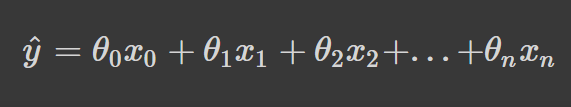
Where θ represents the parameters and n is the number of features.

Essentially, all that occurs in the above equation is the dot product of θ, and x is being summed. Thus, a more concise way to represent this is to use its vectorized form:

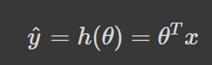
h(θ) is the hypothesis function.

Given this approximate target function, we can use our model to make predictions. To determine if our model has learned well, it’s important we measure the performance of our model on the training data. For this purpose, we compute a loss function. The goal of the training process is to find the values of theta (θ) that minimize the loss function.

Here’s how we can represent our loss function mathematically:

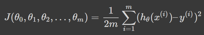
In the above equation, theta (θ) is a n + 1 dimensional vector, and our loss function is a function of the vector value. Consequently, the partial derivative of the loss function, J, has to be taken with respect to every parameter of θ_j in turn. All of them must equal zero. Following this process and solving for all of the values of θ from θ_0 to θ_n will result in the values of θ that minimize the loss function.

Working through the solution to the parameters θ_0 to θ_n using the process described above results in an extremely involved derivation procedure. There is indeed a faster solution.

Take a look at the formula for the normal equation:

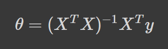
Where:

θ → The parameters that minimize the loss function X → The input feature values for each instance y → The vector of output values for each instance

The Normal Equation vs Gradient Descent

While both methods seek to find the parameters theta (θ) that minimize the loss function, the method of approach differs greatly between the two solutions.

Since we’ve already covered how the normal equation works in ‘What is the Normal Equation?’, in this section, we will briefly touch on gradient descent and then provide ways in which the two techniques differ.

Gradient Descent

Gradient descent is one of the most used machine learning algorithms in machine learning. It’s deployed to iteratively find the parameters theta (θ) that minimize the loss function.

The process starts by first evaluating the model's performance. Next, the partial derivative is calculated from the loss function which is used to reference the slope at its current point. Lastly, we take steps proportional to the negative gradient to make a descent to the minimum of the loss function by updating the current set of parameters - see formula below.

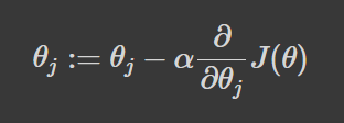
This process is repeated until convergence at the minimum of the loss function.

How do they Differ?

The most obvious way in which the normal equation differs from gradient descent is that it’s analytical. Gradient descent takes an iterative approach which means our parameters are updated gradually until convergence. Another subtle difference baked into this is that gradient descent requires us to define a learning rate that controls the size of the steps taken towards the minimum of the loss function. The normal equation doesn’t require us to define a learning rate because we are not taking iterative steps - we get the results directly.

Also, feature scaling is not required when we use the normal equation approach; we typically perform feature scaling to ensure our features have a similar range of values. This is because gradient descent is sensitive to the ranges of our data points. Failing to normalize our features when we use gradient descent may introduce skewness into the contour plot of the loss function, but the normal equation does not suffer from this problem.

Deciphering When to Use the Normal Equation

The best way to know if you should use the normal equation over gradient descent is to understand its disadvantages.

Computing the normal equation becomes computationally challenging when the number of features in our dataset is large. The reason for this is that in order to solve for the parameters θ, the term (X’ X)^-1 must be computed. Computing X’ X produces an n x n matrix and for most computer implementations, converting a matrix grows approximately as the cube of the dimensions of the matrix. This means the inverse operation runs in O(n^3) runtime complexity which makes the normal equation run extremely slow when n is very large - learn more about time complexity.

Thus, it’s best to use gradient descent when the number of features in the dataset is large. Andrew Ng, a prominent machine learning and AI expert, recommends you should consider using gradient descent when the number of features, n, is greater than 10,000. For 10,000 features or less, you may be better off using the normal equation since you’re not required to select a value for the learning rate which means you have one less hyperparameter to tune.

The Normal Equation from Scratch in Python

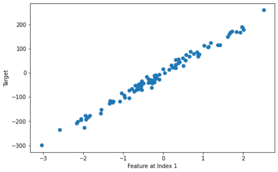
Let’s generate a regression problem to test this equation:

import numpy as np
import matplotlib.pyplot as plt
from sklearn.datasets import make_regression

# Generate a regression problem
X, y = make_regression(
    n_samples=100,
    n_features=2,
    n_informative=2,
    noise = 10,
    random_state=25
    )

# Visualize feature at index 1 vs target
plt.subplots(figsize=(8, 5))
plt.scatter(X[:, 1], y, marker='o')
plt.xlabel("Feature at Index 1")
plt.ylabel("Target")
plt.show()

Here’s where we will implement the normal equation:

# adds x0 = 1 to each instance
X_b = np.concatenate([np.ones((len(X), 1)), X], axis=1)
# calculate normal equation
theta_best = np.linalg.inv(X_b.T.dot(X_b)).dot(X_b.T).dot(y)
# best values for theta
intercept, *coef = theta_best
print(f"Intercept: {intercept}\n\
Coefficients: {coef}")

Intercept: 0.35921242677977794
Coefficients: [6.129199175400593, 96.44309685893134]

Let’s put our model to the test by making a prediction:

# making a new sample
new_sample = np.array([[-2, 0.25]])
# adding a bias term to the instance
new_sample_b = np.concatenate([np.ones((len(new_sample), 1)), new_sample], axis=1)
# predicting the value of our new sample
new_sample_pred = new_sample_b.dot(theta_best)
print(f"Prediction: {new_sample_pred}")
Prediction: [12.21158829]

Whenever you implement a machine learning algorithm from scratch, it’s always helpful to have a method of validating your solution; Scikit-learn is one of the most popular machine learning libraries in Python. It features several implementations of different algorithms, including linear regression, which we will be using to validate our normal equation.

from sklearn.linear_model import LinearRegression

lr = LinearRegression()
lr.fit(X, y)

print(f"Intercept: {lr.intercept_}\n\
Coefficients: {lr.coef_}")
print(f"Prediction: {lr.predict(new_sample)}")

Intercept: 0.3592124267797807
Coefficients: [ 6.12919918 96.44309686]
Prediction: [12.21158829]

The solutions are approximately equal so we can confirm our solution is correct.