Data Manipulation in Excel Cheat Sheet
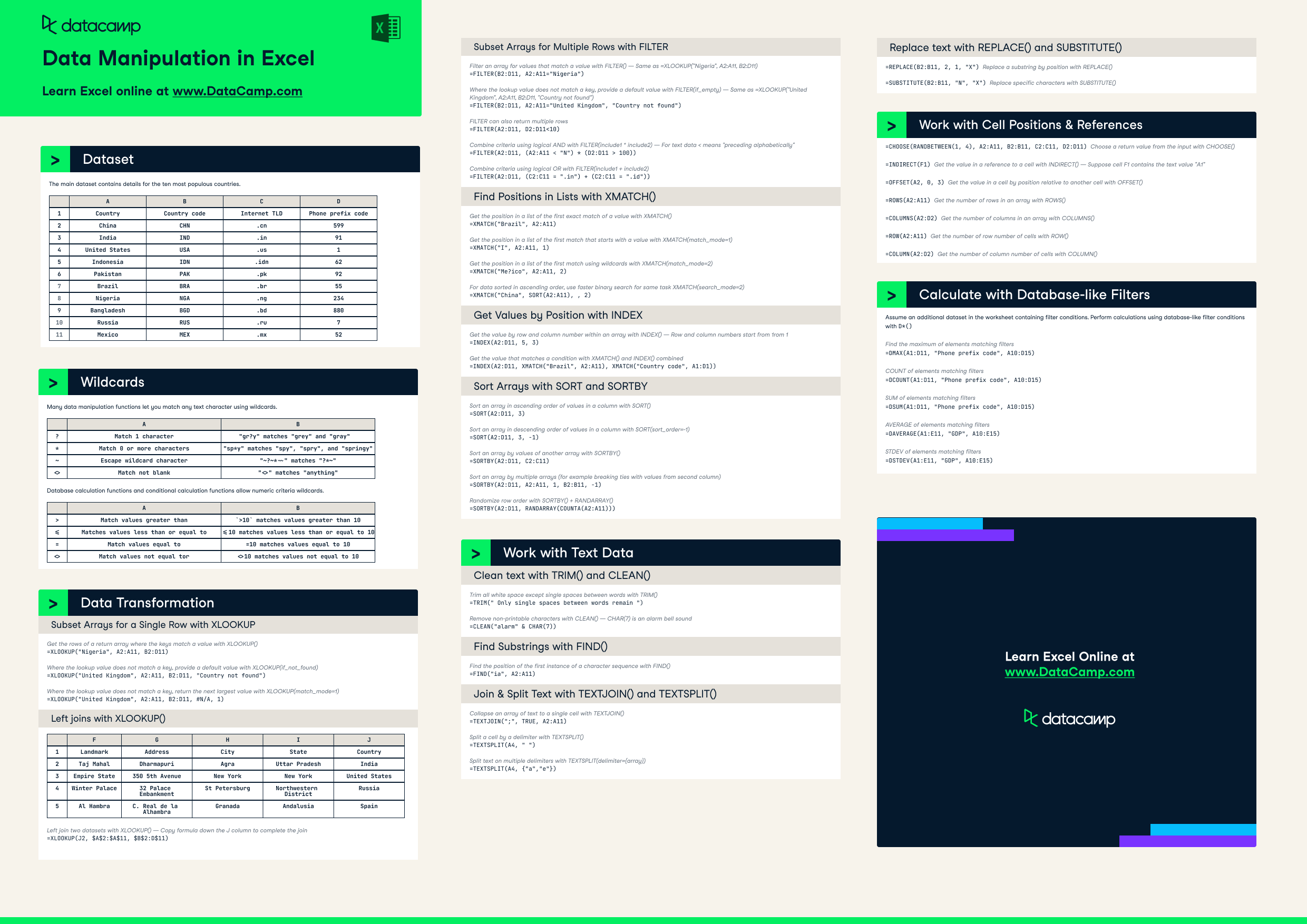
Have this cheat sheet at your fingertips
Download PDFDataset
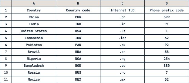
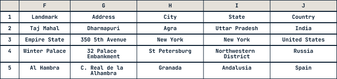
The main dataset contains details for the ten most populous countries.
Wildcards
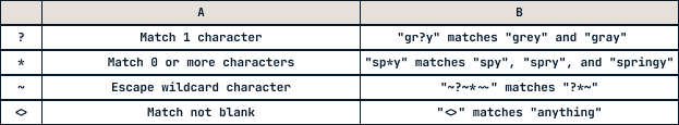
Many data manipulation functions let you match any text character using wildcards.
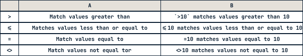
Database calculation functions and conditional calculation functions allow numeric criteria wildcards.
Data Transformation
Subset Arrays for a Single Row with XLOOKUP
Get the rows of a return array where the keys match a value with XLOOKUP()
=XLOOKUP("Nigeria", A2:A11, B2:D11)
Where the lookup value does not match a key, provide a default value with XLOOKUP(if_not_found)
=XLOOKUP("United Kingdom", A2:A11, B2:D11, "Country not found")
Where the lookup value does not match a key, return the next largest value with XLOOKUP(match_mode=1)
=XLOOKUP("United Kingdom", A2:A11, B2:D11, #N/A, 1)
Left joins with XLOOKUP()
Left join two datasets with XLOOKUP() — Copy formula down the J column to complete the join
=XLOOKUP(J2, $A$2:$A$11, $B$2:D$11)
Subset Arrays for Multiple Rows with FILTER
Filter an array for values that match a value with FILTER() — Same as
=XLOOKUP("Nigeria", A2:A11, B2:D11)=FILTER(B2:D11, A2:A11="Nigeria")
Where the lookup value does not match a key, provide a default value with FILTER(if_empty) — Same as =XLOOKUP("United Kingdom", A2:A11, B2:D11, "Country not found")
=FILTER(B2:D11, A2:A11="United Kingdom", "Country not found")
FILTER can also return multiple rows
=FILTER(A2:D11, D2:D11<10)
Combine criteria using logical AND with FILTER(include1 * include2) — For text data < means "preceding alphabetically"
=FILTER(A2:D11, (A2:A11 < "N") * (D2:D11 > 100))
Combine criteria using logical OR with FILTER(include1 + include2)
=FILTER(A2:D11, (C2:C11 = ".in") + (C2:C11 = ".id"))
Find Positions in Lists with XMATCH()
Get the position in a list of the first exact match of a value with XMATCH()
=XMATCH("Brazil", A2:A11)
Get the position in a list of the first match that starts with a value with XMATCH(match_mode=1)
=XMATCH("I", A2:A11, 1)
Get the position in a list of the first match using wildcards with XMATCH(match_mode=2)
=XMATCH("Me?ico", A2:A11, 2)
For data sorted in ascending order, use faster binary search for same task XMATCH(search_mode=2)
=XMATCH("China", SORT(A2:A11), , 2)
Get Values by Position with INDEX
Get the value by row and column number within an array with INDEX() — Row and column numbers start from 1rom 1
=INDEX(A2:D11, 5, 3)
Get the value that matches a condition with XMATCH() and INDEX() combined
=INDEX(A2:D11, XMATCH("Brazil", A2:A11), XMATCH("Country code", A1:D1))
Sort Arrays with SORT and SORTBY
Sort an array in ascending order of values in a column with SORT()
=SORT(A2:D11, 3)
Sort an array in descending order of values in a column with SORT(sort_order=-1)
=SORT(A2:D11, 3, -1)
Sort an array by values of another array with SORTBY()
=SORTBY(A2:D11, C2:C11)
Sort an array by multiple arrays (for example breaking ties with values from second column)
=SORTBY(A2:D11, A2:A11, 1, B2:B11, -1)
Randomize row order with SORTBY() + RANDARRAY()
=SORTBY(A2:D11, RANDARRAY(COUNTA(A2:A11)))
Work with Text Data
Clean text with TRIM() and CLEAN()
Trim all white space except single spaces between words with TRIM()
=TRIM(" Only single spaces between words remain ")
Remove non-printable characters with CLEAN() — CHAR(7) is an alarm bell sound
=CLEAN("alarm" & CHAR(7))
Find Substrings with FIND()
Find the position of the first instance of a character sequence with FIND()
=FIND("ia", A2:A11)
Join & Split Text with TEXTJOIN() and TEXTSPLIT()
Collapse an array of text to a single cell with TEXTJOIN()
=TEXTJOIN(";", TRUE, A2:A11)
Split a cell by a delimiter with TEXTSPLIT()
=TEXTSPLIT(A4, " ")
Split text on multiple delimiters with TEXTSPLIT(delimiter={array})
=TEXTSPLIT(A4, {"a","e"})
Replace text with REPLACE() and SUBSTITUTE()
=REPLACE(B2:B11, 2, 1, "X") Replace a substring by position with REPLACE()
=SUBSTITUTE(B2:B11, "N", "X") Replace specific characters with SUBSTITUTE()
Work with Cell Positions & References
=CHOOSE(RANDBETWEEN(1, 4), A2:A11, B2:B11, C2:C11, D2:D11) Choose a return value from the input with CHOOSE()
=INDIRECT(F1) Get the value in a reference to a cell with INDIRECT() — Suppose cell F1 contains the text value "A1"
=OFFSET(A2, 0, 3) Get the value in a cell by position relative to another cell with OFFSET()
=ROWS(A2:A11) Get the number of rows in an array with ROWS()
=COLUMNS(A2:D2) Get the number of columns in an array with COLUMNS()
=ROW(A2:A11) Get the number of row number of cells with ROW()
=COLUMN(A2:D2) Get the number of column number of cells with COLUMN()
Calculate with Database-like Filters
Assume an additional dataset in the worksheet containing filter conditions. Perform calculations using database-like filter conditions with D*()
Find the maximum of elements matching filters
=DMAX(A1:D11, "Phone prefix code", A10:D15)
COUNT of elements matching filters
=DCOUNT(A1:D11, "Phone prefix code", A10:D15)
SUM of elements matching filters
=DSUM(A1:D11, "Phone prefix code", A10:D15)
AVERAGE of elements matching filters
=DAVERAGE(A1:E11, "GDP", A10:E15)
STDEV of elements matching filters
=DSTDEV(A1:E11, "GDP", A10:E15)
Master your data skills with DataCamp
More than 10 million people learn Python, R, SQL, and other tech skills using our hands-on courses crafted by industry experts.

cheat sheet
Excel Shortcuts Cheat Sheet

Richie Cotton
4 min
cheat sheet
Excel Formulas Cheat Sheet
Richie Cotton
18 min
cheat sheet
Data Transformation with Power Query M in Power BI
Richie Cotton
9 min
cheat sheet
Working with Tables in Power Query M in Power BI
Richie Cotton
6 min
tutorial
How to Clean Data in Excel: A Beginner's Guide

Laiba Siddiqui
15 min
tutorial
Getting Started with Spreadsheets

Ryan Sheehy
5 min