Data Structures: A Comprehensive Guide With Python Examples

Data structures exist in both the digital and physical worlds. A dictionary is a physical example of a data structure where the data comprises word definitions organized in alphabetical order within a book. This organization allows for a specific query: given a word, one can look up its definition.

At its core, a data structure is a method of organizing data that facilitates specific types of queries and operations on that data.

We'll begin by covering linear data structures like arrays, lists, queues, and stacks. We'll then circle back to explain the difference between linear and non-linear structures before diving into hash tables, trees, and graphs.

If you want to learn more, check out this course on data structures and algorithms in Python.

Arrays

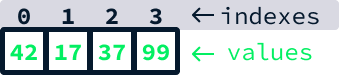
Arrays are fundamental data structures widely available across programming languages. They enable the storage of a fixed number (N) of values sequentially in memory.

Array elements are indexed from the first element at index (0) to the last element at index (N-1).

They allow the following operations:

1. Read the value at a given index.
2. Update the value at a given index.
3. Iterate over all stored values.
4. Obtain the size of the array.

Arrays are highly effective in scenarios where the number of values to be stored is known in advance, and the primary operations involve reading and writing data at specific indexes.

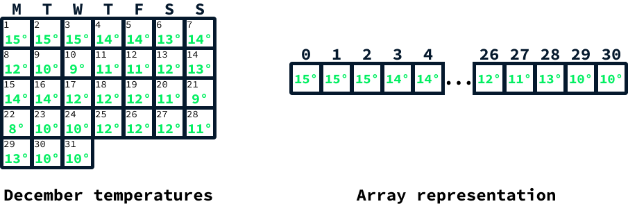
Consider a scenario in which you need to store daily temperature readings for the month of December. You might want to enable users to retrieve the temperature for a specific day and perform various statistical analyses on the temperatures throughout the month.

Since the number of days in December is known in advance to be 31, arrays are an excellent choice for storing the temperature readings. Initially, one would create an array with 31 empty positions. Then, after obtaining each temperature reading, the temperature for a given day would be assigned to the corresponding array index: day 1 would be stored at index 0, day 2 at index 1, and so on, until day 31, which would be stored at index 30.

Accessing the corresponding index allows retrieval of the temperature for a specific day. Statistics, such as the average temperature, can be determined by iterating over all elements, maintaining a cumulative sum, and then dividing by the array's size.

Arrays are not natively available in Python. They are used behind the scenes as the underlying structure for various data types but are not directly supported in the language. To use arrays explicitly, one can utilize libraries such as array, which offer an array implementation. However, it's often more practical to use a list with a fixed size in situations where an array might be required. Lists offer flexibility and are a core part of Python's functionality, as we'll discuss next.

We can create a list to simulate an array of 31 elements, each initialized to None, by using [None] * 31. Here, None indicates that no temperature reading has been recorded yet.

december_temperatures = [None] * 31

To set the value at a specific index, we use december_temperatures[index], where index is a number from 0 to 30. For example, to record the temperature for the first day (stored at index 0), we would do it like this:

december_temperatures[0] = 15

Accessing a temperature is similarly straightforward, using december_temperatures[index].

print(december_temperatures[0])

15

Lists

Imagine now that, instead of focusing on December, we install a sensor somewhere to take periodic temperature readings over an unspecified period. In this scenario, using an array isn't the best option because we might run out of space due to its fixed size upon creation.

A more suitable data structure in this scenario would be a list. There are two kinds of lists:

• Array lists
• Linked lists

Array lists

Array lists can be seen as a more flexible version of arrays. They can perform all the functions that arrays do but also append new values, so their size isn't fixed upon creation. Array lists correspond to using list() in Python.

Their implementation relies on using an array that's expanded when space runs out, hence the name array list. However, as we learned earlier, arrays cannot grow, so how is this possible?

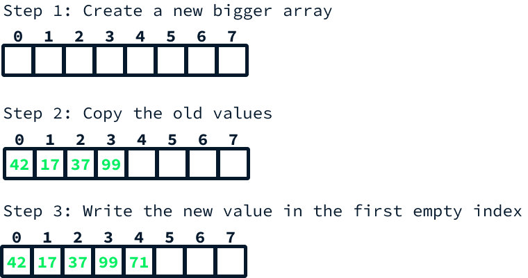
When the underlying array of an array list is full, and we want to append a new value, a larger array is created under the hood. All the previous values are copied into this new, bigger array. Then, the new value is added at the first available position in the new array.

Imagine we want to append the value 71 to this array:

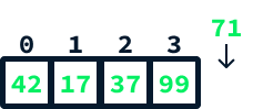
This can be accomplished like so:

The amount of new space allocated whenever we perform this operation is crucial to the performance of the array list. If, at each append, we created an array with just one new position for the new value being appended, it would mean that each append operation would require copying the entirety of the pre-existing data. This would be extremely inefficient—imagine having to copy millions of records simply to add a new one.

Instead, the common strategy is to double the array size each time more space is needed. This approach can be shown to nullify the effect of having these extra copy steps over time.

To add elements to a Python list, we use the .append() method. Here is an example of how to create an empty list and add a temperature reading to it:

temperatures = []
temperatures.append(35)

Linked lists

To structure data in a computer, we need a way to relate values to one another. Arrays accomplish this by allocating contiguous memory locations – meaning memory locations directly next to each other – and storing values sequentially. Think of it as a row of houses on a street: each house has a unique address (index), and they are physically located next to one another.

However, this is not the sole method for organizing data. An alternative involves using a node-based structure.

A node is an object that stores a value along with references to other nodes. For instance, to create a list-like structure using nodes, we can have a node that holds both a value and a reference to the next element in the list. In Python, this can be implemented with a class:

class Node:
    def __init__(self, value, next_node):
        self.value = value
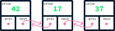
        self.next_node = next_node

Using this approach, one can create a list by linking values together through the next_node reference. Here's a snippet of code that creates a list with the values 42, 17, and 37:

node_37 = Node(37, None) # There's no node after 37 so next_node is None
node_17 = Node(17, node_37)
node_42 = Node(42, node_17)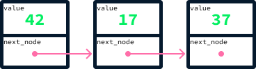

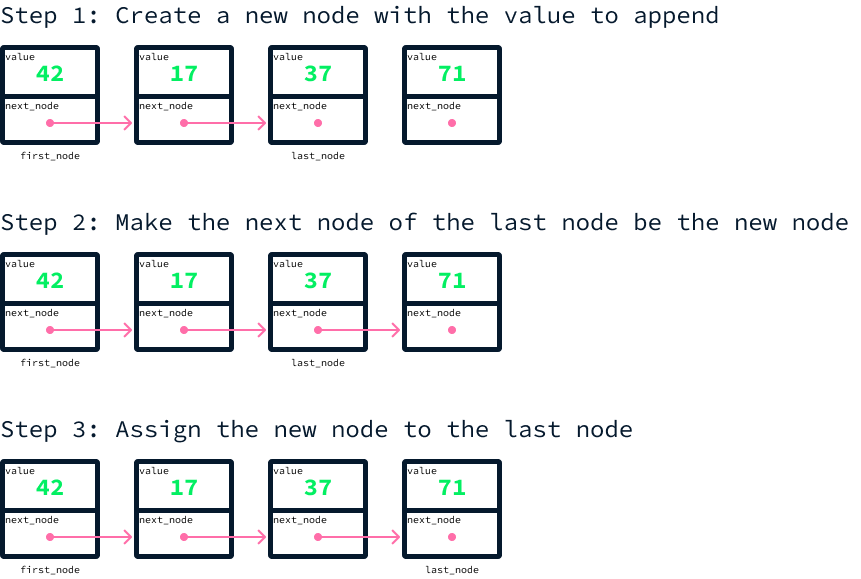
Manually linking nodes in this manner is not practical. The actual implementation requires creating another class that maintains references to both the first and last nodes of the list. To append a new value, we:

1. Create a node with the desired value.
2. Set this new node as the next node of the current last node.
3. Update the reference of the last node to this newly added node.

Imagine we want to append the value 71 to our example array:

This can be accomplished like so:

class LinkedList:
    def __init__(self):
        self.first_node = None
        self.last_node = None

    def append(self, value):
        node = Node(value, None)
        if self.first_node is None:
            self.first_node = node
            self.last_node = node
        else:
            self.last_node.next_node = node
            self.last_node = node

Unlike in array lists, we cannot directly access values by their indices. To read a specific value at an index, we must start from the first node and sequentially move from one node to the next until we reach the desired index. This process is significantly slower than direct access. If we have millions of values stored in the list, we would need to read through millions of values in memory to reach a specific index.

The advantage of a linked list lies in the fact that we can instantly add and remove elements from either the front or the back of the list. This capability opens up the possibility of implementing two new data structures: queues and stacks, which we'll discuss next.

Queues

Imagine you're developing a restaurant app that logs customer orders and forwards them to the kitchen. When customers arrive at the restaurant, they will queue up to place their orders, expecting to be served in the sequence of their arrival. This means that the first customer in line should receive their order first, and the last customer in line should receive their order last.

In the kitchen, the chef prefers to focus on one order at a time, so the app should only display the current order. Once an order is prepared and dispatched, the next order in the queue should be displayed.

We can interpret the above requirements as needing a data structure that supports the following operations:

1. Adding elements.
2. Viewing the element that has been added first.
3. Removing the element that has been added first.

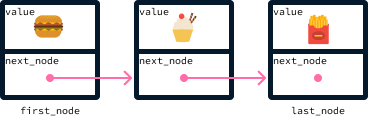
These operations are precisely what a queue offers. A queue can be implemented using a linked list, where elements are added by appending them to the list. Since elements are ordered by their arrival time, the first node is always the one that should be served next.

Here's how the orders above would be stored in the queue:

Once an order is ready, it can be removed by updating the first element to its next_node, assuming there is a subsequent node. The new first node becomes the second node:

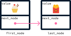
Queues are described as a first-in, first-out (FIFO) data structure because the first element to be added is also the first to be removed. In our restaurant example, the first customer to arrive is also the first to be served (and removed from the chef’s list).

To use a queue in Python, we can utilize the deque collection from the collections module. Import this module and create an empty queue as shown below:

from collections import deque
orders = deque()

Adding a new element to the back of the queue can be achieved using the .append() method:

orders.append("burger")
orders.append("sunday")
orders.append("fries")

To retrieve and remove the next order from the front of the queue, we use the .popleft() method:

orders.append("burger")
orders.append("sunday")
orders.append("fries")

burger
sunday
fries

Stacks

In certain situations, we desire the opposite of a queue's behavior—we rather want to track the most recently added element.

To exemplify this, imagine you're tasked with adding an undo feature to an image editor. This requires a method to monitor the user’s actions, providing access to the most recent operations. This is because undo functionalities typically reverse actions starting from the last one performed and moving towards the first.

A stack is exactly a data structure that supports these operations:

1. Adding elements.
2. Viewing the element that was last added.
3. Removing the element that was last added.

Like queues, stacks can also be implemented using a linked list. Adding an element is still accomplished by appending the element to the list. However, our interest shifts to the last element of the list instead of the first. To retrieve the most recent element, we look up the last element of the list. Removing the last element requires us to delete the last element.

In our node structure, we only tracked the next node. To facilitate the removal of the last element, we need to access the element that precedes it, delete its next_node, and promote that node to be the last. We can accomplish this by modifying the node structure to also track the previous node of each node. Such a linked list is referred to as a doubly linked list.

Stacks are described as a last-in, first-out (LIFO) data structure because the last element to be added is also the first to be removed.

To use a stack in Python, we can utilize the same deque collection. We use the .append() method to add new elements:

from collections import deque
actions = deque()

actions.append("crop")
actions.append("desaturate")
actions.append("resize")

To retrieve and remove the next order from the top of the stack, we use the .pop() method:

print(actions.pop())
print(actions.pop())
print(actions.pop())

resize
desaturate
crop

Linear vs. Non-linear Data Structures

So far, we’ve explored five data structures: arrays, array lists, linked lists, queues, and stacks. Each of these is a linear data structure because their elements are arranged in a sequence, with each element having a clear previous and next element.

Next, we'll shift our focus to non-linear data structures. Unlike linear types, these structures don’t organize elements next to each other in a linear fashion. Consequently, they don’t have a defined notion of previous and next elements. Instead, they establish different types of relationships among the elements.

This characteristic makes them particularly suitable for executing specialized queries on the data with high efficiency rather than merely serving as a means of storing data in memory.

Hash tables

We started this article by discussing a real-life example of a data structure: dictionaries. It turns out that organizing data so that it can be looked up by a specific field (for example, looking up a definition given a word) is extremely useful in general, so computer scientists also invented a data structure that enables this.

To understand this data structure, let's see how we can create a virtual dictionary—that is, a data structure where we can:

1. Add a word at its definition.
2. Given a word, look up its definition.

Recall the example of recording temperatures throughout December. We used an array with 31 elements corresponding to each day of the month to store the temperatures at their respective indexes. This approach allows for the efficient lookup of the temperature for any given day.

This scenario is akin to dealing with data pairs (day, temperature), where the objective is to retrieve the temperature by specifying the day. Similarly, in the case of dictionaries, we handle data pairs (word, definition) and aim to find the definition when provided with a word.

Such pairs are referred to as key-value pairs or entries. The key is the parameter used in the lookup query, and the value is the outcome of that query.

What prevents us from using an array for the dictionary problem is that our keys are strings rather than numbers. With numeric keys, we can directly use an array to associate keys and values by positioning the values at their corresponding indexes.

To solve this problem, we first need to convert the words into numbers. A function that performs this conversion is referred to as a hash function. There are numerous approaches for creating such a function. For instance, we could assign numeric values to letters, with a as 1, b as 2, c as 3, and so forth, then sum these values.

For example, the word data would be calculated as 4 + 1 + 20 + 1 = 26. However, this function has its drawbacks, which we'll discuss shortly. The details on how to devise an effective hash function are beyond the purpose of this article, but Python conveniently provides a hash() function that efficiently handles this task for us.

hash("data")

-6138587229816301269

In the above example, you might have observed that the hash function produced a negative number. It's important to note that array positive indices range from 0 to N - 1. Once we have converted keys into numbers, we can map them to the 0 to N - 1 range using the modulo operator % (which outputs the remainder of a division—for instance, 10 % 3 outputs 1).

As a side note, Python’s hash() function may return different values across different program executions. It's only deterministic within the same program run, meaning you may observe different hash values for the same object if you execute your program multiple times.

Consider an array that contains 100 elements. To locate the index corresponding to the string "data", we proceed as follows:

hash("data") % 100

31

The hash table data structure is essentially a large array that stores key-value pairs at indexes determined by applying a hash function to the keys.

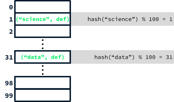
Because of space constraints, the diagram above only includes the abbreviation "def" to represent the definition. However, in practice, each entry's second element would be the word's full definition.

There's another important aspect to consider. Given that there are significantly more than 100 words, if we continue adding words, distinct words will inevitably yield the same hash value. To solve this, instead of limiting each array element to a single key-value pair, we employ a linked list to store all entries sharing the same hash value.

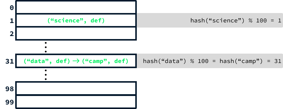
When two entries generate the same hash, this is called a collision. This scenario slightly modifies the lookup process. After computing the hash code, it's necessary to traverse the list to locate the correct entry. While this approach slows down the lookup operation, it can be demonstrated that using a sufficiently large initial array size (larger than 100) and a well-designed hash function can significantly mitigate the impact of collisions. Consequently, the efficiency remains nearly equivalent to that of an array.

For an effectively designed hash function, finding distinct values that result in the same hash should be rare. This is why a simplistic hash function that merely adds up the numerical values of the characters in a word is not ideal. Any two words composed of the same letters, regardless of their order, would yield identical hash codes. For instance, “listen” and “silent” would produce the same hash. In contrast, the built-in hash function provided by Python is significantly more robust and is specifically engineered to minimize collisions.

Hash tables are arguably the most important data structure available. They are extremely efficient and versatile. In Python, they are implemented through the dict() class. Due to its resemblance to a dictionary, in Python, the data structure is actually called a dictionary instead of a hash table.

For the sake of simplicity, our example focuses on adding and looking up entries. Generally, dictionaries offer more flexibility and support additional operations, including deletion. To create an empty dictionary (hash table) in Python, you can use {} like this:

word_definitions = {}
word_definitions["data"] = "Facts or information."

You can access a word's definition by using the word as the key, like this:

print(word_definitions["data"])

Facts or information.

Trees

Imagine you're developing a website for a real estate agency. Your task is to create a feature that allows users to filter listings by price. The feature should allow users to:

1. Find the cheapest listing.
2. Find the most expensive listing.
3. Find all listings below a given price.

Typically, this process would involve traversing all house listings and filtering out the ones that fall outside the desired price range. However, our goal is to develop a solution that scales more efficiently, one that does not require examining the entire dataset to find relevant listings. Trees are the perfect data structure to answer this kind of query.

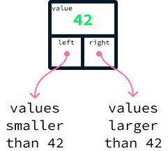
Trees are node-based data structures, like linked lists. However, instead of having previous and next references, each node will keep a value and two references: a left node and a right node.

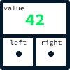
In our real estate agency website example, each node will represent a property listing. To optimize price-related queries, we'll establish a rule: listings with lower prices will always be stored to the left of a node, while listings with higher prices will always be stored to the right.

For a concrete example, consider the following tree holding the values 42, 17, 73, 4, 22, and 89.

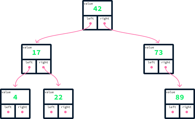
For each node, all the nodes on the left have smaller values, and all those on the right have larger values. A tree satisfying this property is called a binary search tree (BST). It's binary because each node refers to at most two other nodes, called children. The search part of the term comes from the fact that the ordering property on the left and right children will make it possible to search the tree efficiently.

We can already see how a BST helps quickly find the cheapest and most expensive listings. Because of the value ordering, the cheapest is always the leftmost node, and the most expensive is always the rightmost node.

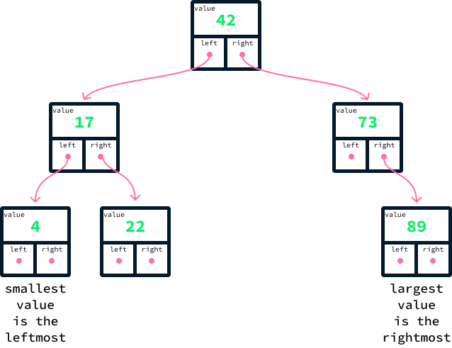
This implies that we can locate them without examining most of the data. Beginning at the top node, also called the root node, we consistently follow the left links to identify the minimum and the right links to identify the maximum. This means that only the nodes along the path connecting the root to the minimum and maximum nodes, respectively, need to be inspected.

Imagine we want to find all nodes with a value of at least 50. These are the steps we can take to accomplish this:

• Starting at the root, we compare our target, 50, with the root's value, which is 42.
• Observing that 50 is larger, we understand that the root and all nodes to its left contain smaller values. Consequently, we can disregard them.
• We then proceed to the node to the right of the root, which is 73. Upon comparison, we find that 50 is smaller than 73. This indicates that all nodes to the right of node 73 meet our criteria.
• However, since 73 doesn’t have a left child, our search concludes there.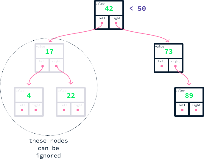

We can already see how BSTs can significantly speed up queries. Even in this small example, we avoided examining half of the data.

Generally, identifying all nodes in a BST that fit into a given range requires inspecting several nodes that are close to the number of query results. This is a huge advantage compared to having to inspect every single data point. Imagine having 1,000,000 listings and a query that yields only 10 results. Using a list, one would have to inspect one million listings to filter out those that don't fit the range. With a BST, one only needs to inspect about 10 listings. This represents a speedup factor of 100,000.

The efficiency of a BST is highly dependent on the balance of the tree. If we add the same values as before, from smallest to largest—4, 17, 22, 42, 73, followed by 89—we could end up with an unbalanced tree, as shown:

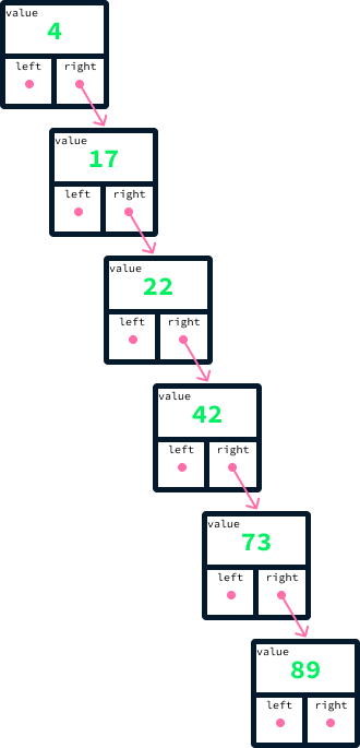
Recall that, to find the maximum value in a BST, we begin at the root and trace the right links until we arrive at a node that does not have one. In the case of an unbalanced tree, such as the one illustrated in the diagram above, this process necessitates examining every single node. Ideally, we aim for the nodes to be evenly distributed between the left and right sides. Explaining the specifics of how this balancing can be consistently achieved falls outside the scope of this article. A type of binary search tree known for maintaining such balance is called an AVL tree.

The avltree package provides an implementation of an AVL tree. The code snippet below shows how we can use it on this house listing dataset, a cleaned subset of this USA Real Estate Dataset.

import csv
from avltree import AvlTree as Tree

# Load the listings CSV data
with open("listings.csv", "rt") as f:
    reader = csv.reader(f)
    listings = list(reader)

# Create the tree based on the price column (column index 2)
tree = Tree()
for listing in listings[1:]:
    price = float(listing[2])
    tree[price] = listing

# Display the cheapest listing price
print("Cheapest:", tree.minimum())

# Display the most expensive listing price
print("Most expensive:", tree.maximum())

# Display the number of listings whose price is between 100,000 and 110,000
listings_in_range = list(tree.between(100000, 110000))
print("Num listings between 100000 and 110000:", len(listings_in_range))

Cheapest: 50017.0
Most expensive: 19999900.0
Num listings between 100000 and 110000: 403

We first use the csv module to read the listings.csv dataset. Subsequently, we create an AVL tree based on the price column. We then use the minimum(), maximum() and between() methods to determine the minimum price, maximum price, and the number of listings priced between $100,000 and $110,000.

Graphs

The final data structure we’ll discuss in this article is the graph.

Let’s say you’re analyzing data from a social media platform. This data comprises a list of users and the friendships between them, and your goal is to identify communities within the social network. Although the concept of a community can be defined in various ways, it generally refers to a group of users who have a significant number of friendships within that group.

Graphs are the ideal data structure for representing data when we have entities and relationships between pairs of these entities. In our example, the entities are users, and the relationships are their friendships.

Graphs are node-based structures. However, unlike linked lists and trees, which exhibit linear or hierarchical connections between nodes, a graph allows any node to connect to multiple other nodes. These connections between nodes, called edges, indicate relationships between them.

In our social network example, each user can be visualized as a node. An edge can be drawn between two nodes to denote a friendship between the corresponding users.

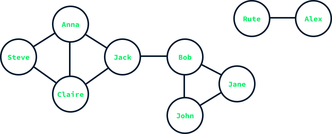
The diagram above illustrates a graph representing friendships within a small social network. The nodes represent the users and are labeled with their names, while the edges represent the friendships. For example, Anna is friends with Steve, Claire, and Jack, which means there are edges connecting her node to the nodes of these individuals.

The operations that a graph data structure should support include:

1. Adding a new node.
2. Connecting two nodes with an edge.
3. Retrieving all nodes connected to a specific node.

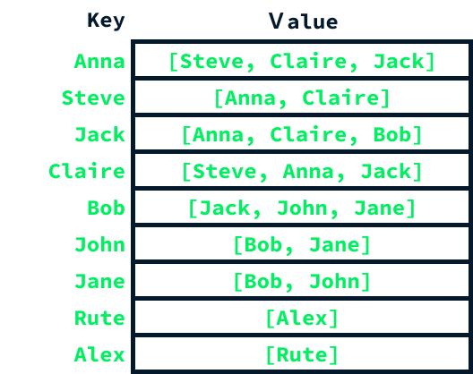
A common way of implementing a graph is by using a hash table and lists. A hash table is created with one entry for each node. The key of each entry is the node, and the value is a list containing all the nodes to which that node is connected.

The networkx package offers a Python implementation for creating and manipulating graphs. Moreover, the networkx library encompasses a wide array of graph algorithms, including those for community detection. Let's utilize it to construct the graph mentioned earlier and apply a prevalent community detection algorithm to observe the outcomes.

To initiate the graph creation, we begin by importing the networkx library and initializing an empty graph:

import networkx as nx
G = nx.Graph()

Nodes can be added using the add_node() method.

G.add_node("Anna")
G.add_node("Steve")
G.add_node("Jack")
G.add_node("Claire")
G.add_node("Bob")
G.add_node("Jane")
G.add_node("John")
G.add_node("Rute")
G.add_node("Alex")

Edges can be added using the add_edge() method.

G.add_edge("Anna", "Steve")
G.add_edge("Anna", "Jack")
G.add_edge("Anna", "Claire")
G.add_edge("Steve", "Claire")
G.add_edge("Claire", "Jack")
G.add_edge("Jack", "Bob")
G.add_edge("Bob", "John")
G.add_edge("Bob", "Jane")
G.add_edge("John", "Jane")
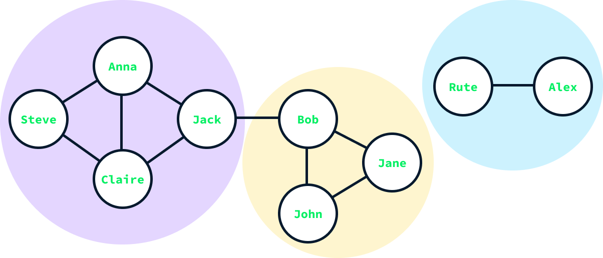
G.add_edge("Rute", "Alex")

With our graph created, we can calculate the communities within it. Several algorithms are designed for community detection, and in this instance, we'll be using the Louvain method. The community detection algorithms can be found in the community subpackage of networkx. Specifically, we'll focus on the louvain_communities() function.

Here's how to utilize it:

communities = nx.community.louvain_communities(G)
print(communities)

[{'Jack', 'Claire', 'Anna', 'Steve'}, {'Bob', 'John', 'Jane'}, {'Rute', 'Alex'}]

The output is a list of sets, with each set representing a community. We observe that the algorithm has detected three communities, which matches our expectations given the structure of the graph.

To learn more about graphs, learn how to implement the Dijkstra algorithm in Python.

Choosing the Right Data Structure

When introducing each data structure, we presented a list of supported operations. These operations serve as guidelines for when to use that data structure, as it's designed to perform these operations efficiently.

For example, the Python list() also supports additional operations, such as removing elements. However, these extra operations are not what an array list excels at. Specifically, removing an element from the middle of a list requires copying all the data (except for the removed element) into a new list, which can be very time-consuming.

When the data is naturally indexed with numbers, and the number of entries is known (for instance, the days of a month), an array is usually the preferred choice. For more generic indexing or dynamic data sets, dictionaries are a good alternative solution.

To process data sequentially, one entry at a time, queues, or stacks are often used, depending on the desired order of data processing.

Trees are typically the answer when we want to perform more complex queries on the data, such as finding all entries within a given range or extremes.

Finally, when there's a relationship between pairs of data points, a graph is an effective way to store and represent these relationships. There are graph algorithms that enable us to answer common questions about datasets with this kind of pairwise relationship.

Data structures constitute a vast domain, and we've only covered the tip of the iceberg. In certain situations, the solution is to design a brand-new data structure fully tailored to the problem at hand. Nevertheless, being familiar with the data structures discussed in this article should point you in the right direction when solving your data-related problems.

Conclusion

In this article, we've learned that data structures are methods of organizing data in particular formats to facilitate efficient information retrieval.

There are two fundamental types of data structures: array-based (for example, hash tables) and node-based (for example, graphs) structures.

Linear structures, such as arrays, queues, and stacks, organize elements sequentially, one after another. In contrast, non-linear structures, such as hash tables, trees, and graphs, organize data based on the relationships within the data.

The choice of the appropriate data structure depends on the nature of the queries to be performed.

If you want to learn about the various data structures in Python, check out this tutorial on Python data structures.