A considerable proportion of the data generated every day is inherently spatial. From Earth Observation data and GPS data to data included in all kinds of maps, spatial data –also known sometimes as geospatial data or geographic information– are data for which a specific location is associated with each record.
Every spatial data point can be located on a map. This can be done using a certain coordinate reference system, for example, the geographical coordinates, which is based on the usual latitude-longitude pairs we use to specify where something is on the globe. This allows us to look at spatial relationships between the data.
Yet, the real power of geospatial data is combining both the data themselves and their location, unlocking several opportunities for sophisticated analysis. The so-called geospatial data science is a subfield of data science that focuses on extracting information from geospatial data by leveraging the power of spatial algorithms and analytical techniques, such as machine learning and deep learning. In other words, geospatial data science helps us understand where things happen and why they happen there.
There are many tools suited for geospatial data science. This tutorial will focus on GeoPandas, an open-source package for working with geospatial data in Python.
GeoPandas extends the datatypes used by pandas –the standard tool for manipulating dataframes in Python– to allow spatial operations on geometric types. Since GeoPandas is built on pandas –as well as other popular Python packages for data science, such as matplotlib–, it’s very easy for data professionals using Python to get fluent with GeoPandas syntax.
Installing Python GeoPandas
To use Python GeoPandas, you first have to install it, just like any other Python library.
It’s important to note that GeoPandas relies on a stack of open-source geospatial libraries to deliver its full spatial potential, including shapely, fiona, pyproj, and rtree. You have to make sure you install all these dependencies, otherwise, GeoPandas may not work as expected.
To avoid complexities, GeoPandas recommends installing the library using the conda package manager. This means you will first need to install Anaconda. For a guide on how to install and use Anaconda, check out our tutorial.
The advantage of using the conda is that it provides pre-built binaries for all the required and optional dependencies of GeoPandas for all operating systems (Windows, Mac, Linux). To install GeoPandas on the command line:
>>conda install geopandasAlternatively, you can install Anaconda using pip, the standard package installer in Python. As already mentioned, you will need to install the required dependencies as well. If you are not familiar with pip, we highly recommend you to read our Pip Python Tutorial for Package Management. The instruction you will have to run to install GeoPandas with pip is:
>>pip install geopandas In any case, if you have troubles during the installation of GeoPandas, you should check the documentation for further information.
Once you have installed the package, you’re set to start using GeoPandas. Just import it into your Python environment. Note that it’s very common to import GeoPandas using the alias gpd.
import geopandas as gpdBasic Operations with GeoPandas
In the section, we will cover the most basic operations you can do with GeoPandas. In doing so, we will introduce you to some critical concepts in geospatial analysis, including types of spatial data, spatial data formats, and coordinate reference systems (CRS).
Reading and writing spatial data
Just like pandas require input data to convert into a pandas dataframe, GeoPandas reads input (spatial) data and converts it into the so-called GeoDataFrame.
Before going into the multiple spatial filetypes GeoPandas can read, it’s important to distinguish the different types of spatial data. The type of data we are dealing with informs what tools we should use to analyze and then visualize the data.
Basically, there are two main types of spatial data:
- Vector data. It describes the features of geographic locations on Earth through the use of discrete geometries, namely:
- Point. Individual locations, like a building, or a car, with X and Y coordinates.
- Line. A series of connected points describing things like roads or streams.
- Polygon. Formed by a closed line that encircles an area, such as the boundaries of a country. Additionally, when one feature consists of multiple geometries, we call it MultiPolygon.
- Raster data. Encodes the world as a continuous surface represented by a grid, such as the pixels of an image. Each piece of the grid can be either a continuous value (such as an elevation value) or a categorical classification (such as land cover classifications). Classic examples include altitude data or satellite images.
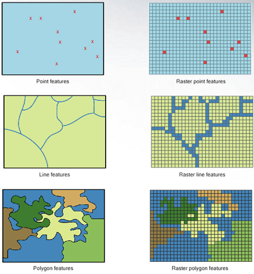
Source: Humboldt State University
Both vector and raster data usually come together with non-spatial data, also known as attributes. Spatial data can have any number of additional attributes accompanying information about the location. For example, the location of a school can be associated with the name of the school, the number of students, or the address.
GeoPandas is designed to work with vector data, although it can easily team up with other Python packages to deal with raster data, like rasterio. To read spatial data, GeoPandas comes with the geopandas.read_file() function. This powerful function can automatically read most of the occurring vector-based spatial data.
Some of the most common vector data formats are:
- Shapefile. As the industry standard, shapefiles are the most common vector data format. It comprises three files that are usually provided in a zip file:
- The .shp file contains shape geometry.
- The .dbf file holds attributes for each geometry,
- The .shx file or shape index file helps link the attributes to the shapes.
- GeoJSON. It’s a newer format for geospatial data released in 2016. Unlike shapefiles, GeoJSON is a single file, making it easier to work with.
In the following examples, we will use the geopandas.read_file() function to read a GeoJSON file hosted in GitHub containing geospatial data about the different districts of the city of Barcelona.
url = 'https://raw.githubusercontent.com/jcanalesluna/bcn-geodata/master/districtes/districtes.geojson'

districts = gpd.read_file(url)

districts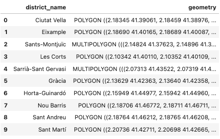
We will go back to this dataset in a minute, but first, you have to know how to write a GeoDataFrame back to a file. It’s fairly easy. You just have to use GeoDataFrame.to_file() to create a file containing the spatial data. By default, the format of the new document will be a shapefile, but you can change it with the “driver” parameter.
For example, you save the district GeoDataFrame into a geoJSON file:
districts.to_file("districts.geojson", driver="GeoJSON")Exploring GeoDataFrames
You may have noticed that the GeoDataFrame in the previous section resembles a traditional pandas dataframe. The similarity makes sense, as GeoDataFrame is a subclass of pandas.DataFrame. That means it inherits many of the methods and attributes of pandas dataframe. What's new in GeoDataFrame is that it can store geometry columns (also known as GeoSeries) and perform spatial operations.
The geometry column can contain any type of vector data, such as points, lines, and polygons. Further, it’s important to note that although a GeoDataFrame can have multiple GeoSeries, only one column is considered the active geometry, meaning that all the spatial operations will be based on that column.
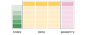
Source: GeoPandas
Another important feature of GeoDataFrames is that every GeoSeries comes with associated CRS information. This CRS information tells GeoPandas where the coordinates are located on Earth. This information is key for spatial analysis. For example, if you need to combine two spatial datasets, you need to make sure they are expressed in the same CRS. Otherwise, you won’t get the result you expected.
There are two main categories of CRS:
- Geographic coordinates. They define a global position in degrees of latitude and longitude relative to the equator and the prime meridian. With this system, we can easily specify any location on earth. It is used widely, for example, in GPS. The most popular CRS is EPSG:4326, also called WGS84.
- Projected coordinates. While Earth is round, we usually represent it on a two-dimension map. Projected coordinates express locations in X and Y dimensions, thereby allowing us to work with a length unit, such as meters, instead of degrees, which makes the analysis more convenient and effective. However, moving from the three-dimensional Earth to a two-dimensional map will inevitably result in distortions. That’s why there are different approaches to creating projected coordinates. For example, many countries have adopted a standard projected CRS for their particular geography.
There’s much more about CRS, but it’s out of the scope of this tutorial. A great resource to get additional information and practical examples is our Working with Geospatial Data in Python Course.
In GeoPandas, the CRS information is stored in the crs attribute:
districts.crs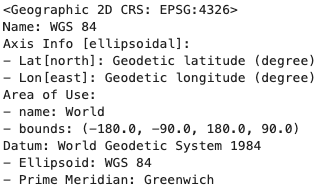
The district GeoDataFrame is associated with geographic coordinates (EPSG: 4326), but we want to transform it into projected coordinates, so we can make some calculations in meters. Let’s transform it to EPSG:2062, the standard projected CRS for Spain. We can do it with the Geopandas.to_crs() method.
districts.to_crs(epsg=2062, inplace=True)

districts.crs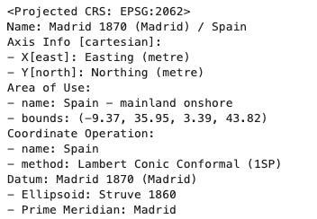
Now that we have set the right projected CRS, we’re ready to explore the attributes of GeoDataFrames.
Exploring the attributes of a spatial dataset
GeoPandas inherits a number of useful methods and attributes from the shapely package. We’re going to cover four of them.
Area
The area attribute returns the calculated area of a geometry. We can save the resulting area (converted to km2) in a new column:
districts['area'] = districts.area / 1000000

districts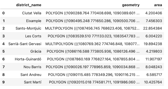
Centroid
The centroid attribute returns the center point of a geometry. We can add it to our dataset, thereby creating a new geometry column.
districts['centroid']=districts.centroid

districts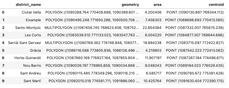
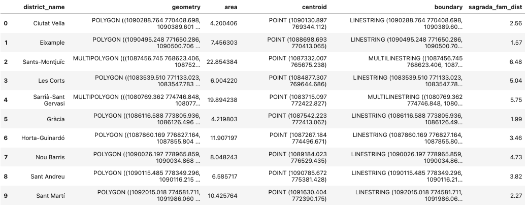
Boundary
The boundary attribute within the boundary of a polygon.
districts['boundary']=districts.boundaryDistance
The distance method gives the minimum distance from a geometry to a location. Say we want to calculate the distance from the famous Sagrada Familia church, located in the Eixample district, to the centroids of every district in Barcelona, and then add the distances (in kilometers) in a new column.

The Sagrada Familia. Source: Wikipedia
First, we need to create a point using the shapely Point() function with the desired coordinates (you can easily find them on Google Maps), convert it into a GeoSeries with the right CRS, and then use the GeoPandas.distance() method:
from shapely.geometry import Point

sagrada_fam = Point(2.1743680500855005, 41.403656946781304)
sagrada_fam = gpd.GeoSeries(sagrada_fam, crs=4326)
sagrada_fam= sagrada_fam.to_crs(epsg=2062)
districts['sagrada_fam_dist'] = [float(sagrada_fam.distance(centroid)) / 1000 for centroid in districts.centroid]
The resulting datasets, following the previous spatial operations, looks like this:
Plotting with GeoPandas
The spatial operations we have performed provide insightful information for our study. However, visualising your geometries in space is a great way to improve your analysis. Fortunately, creating a GeoPandas plot is super easy. You just have to call the GeoDataFrame.plot() function, built upon Python’s matplotlib package.
Let’s start with a basic visualization of Barcelona districts.
ax= districts.plot(figsize=(10,6))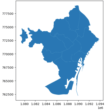
We can make our GeoPandas plot more informative by coloring each district. Setting the legend to 'True' creates a legend to help interpret the colors.
ax= districts.plot(column=district_name', figsize=(10,6), edgecolor='black', legend=True)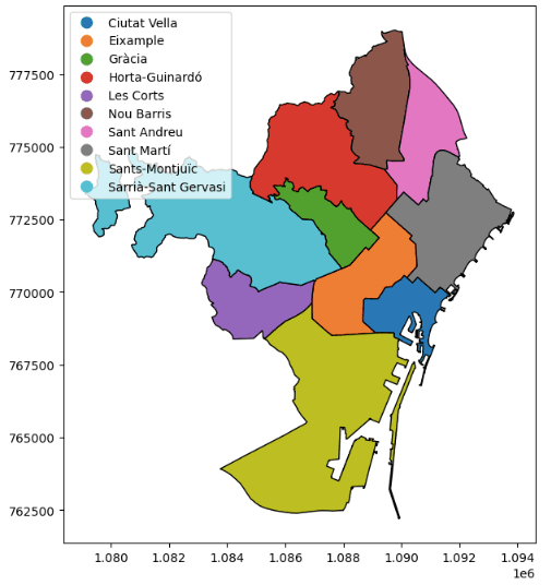
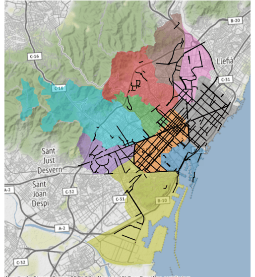
Finally, we can add the centroids of the districts and the Sagrada Familia to our map, as well as a title. Equally, to make the plot more compelling, we can use the nice contextily package to add a tile map of the actual city of Barcelona.
import contextily
ax= districts.plot(column='district_name', figsize=(12,6), alpha=0.5, legend=True)
districts["centroid"].plot(ax=ax, color="green")
sagrada_fam.plot(ax=ax,color='black', marker='+')
contextily.add_basemap(ax, crs=districts.crs.to_string())
plt.title('A Beautiful Map of Barcelona')
plt.axis('off')
plt.show()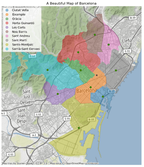
Cool, right? There is much more you can do to make beautiful spatial visualizations. Our course Visualizing Spatial Data With Python is a great resource to take your visualization skills to the next level.
Spatial Relationships with GeoPandas
One of the key aspects of geospatial data is how they relate to each other in space. GeoPandas leverages the power of pandas and shapely packages to perform all kinds of spatial relationships between spatial datasets. In this section, we will cover some of the most common operations.
Attribute Joins
There are two ways to combine datasets in pandas: attribute joins and spatial joins.
Attribute joins allow us to join two GeoDataFrames based on non-geometry variables, just like a regular join in pandas. Indeed, the way to perform attribute joins is through the standard pandas.merge() method. If you are interested in knowing more about pandas joins, check out our Joining DataFrames in pandas tutorial.
For example, it would be interesting to enrich our GeoDataFrame with the population data of Barcelona in 2022.
pop =pd.read_csv('poblacion_barna_2022.csv', usecols=['Nom_Districte','Nombre'])
pop = pd.DataFrame(pop.groupby('Nom_Districte')['Nombre'].sum()).reset_index()
pop.columns=['district_name','population_22']
districts = districts.merge(pop)
districtsv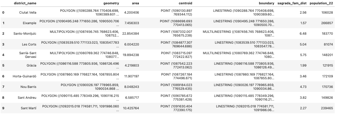
Spatial Joins
By contrast, spatial joins allow the merging of two GeoDataFrames based on their spatial relationships.
For example, let’s identify the districts in which the bicycle lanes in Barcelona are located.
url = 'https://opendata-ajuntament.barcelona.cat/resources/bcn/CarrilsBici/CARRIL_BICI.geojson'
bike_lane = gpd.read_file(url)
bike_lane = bike_lane.loc[:,['ID','geometry']]
bike_lane.to_crs(epsg=2062, inplace=True)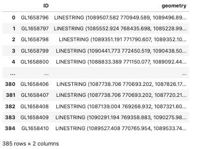
In GeoPandas, the spatial join operation is available as the sjoin() function. The first argument we specify is the GeoDataFrame to which we want to add information, and the second argument is the GeoDataFrame that contains the information we want to add. Then, we have to specify the type of join. Finally, the parameter “predicate” tells GeoPandas which spatial relationship we want to use to match both datasets. Some of the most common relationships “intersects”, “contains”, and “within”.
In our example, we will use the predicate “intersects”. Two geometric objects intersect if they have any boundary or interior point in common.
lanes_districts = gpd.sjoin(districts, bike_lane, how='inner', predicate='intersects')
lanes_districts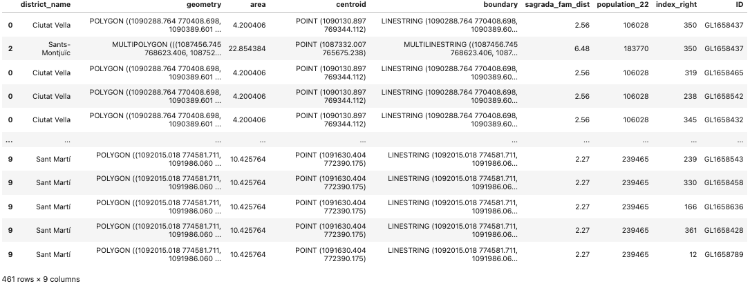
Note that the resulting GeoDataFrame has more rows than the bike_lane GeoDataFrame. That’s because a bike lane may be located in more than one district.
Finally, we can group our dataset to get the number of bike lanes by districts:
lanes_districts.groupby('district_name').size()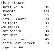
GeoPandas Overlay operations
Finally, spatial overlays allow you to compare two GeoDataFrames containing polygon or multipolygon geometries and create a new GeoDataFrame with the new geometries representing the spatial combination and merged properties. The image below shows the different possibilities:
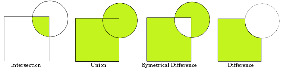
Source: GeoPandas
Image the Barcelona City Council wants to build new local parks in an effort to tackle pollution and promote community wellness. A preliminary idea is to create big, round parks within 500 meters of the center of every district. We can simulate this by creating a buffer based on the centroid of every district.
parks = gpd.GeoDataFrame(districts.centroid.buffer(500), geometry=0)

parks.plot()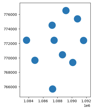
Now, we are ready to perform some overlay operations. For example, if we want to see only the areas of the districts where the parks would be located, we can use the GeoPandas.overlay() method:
parks_intersection = districts.overlay(parks, how='intersection')
ax = parks_intersection.plot(alpha=0.5, edgecolor='black', column='district_name')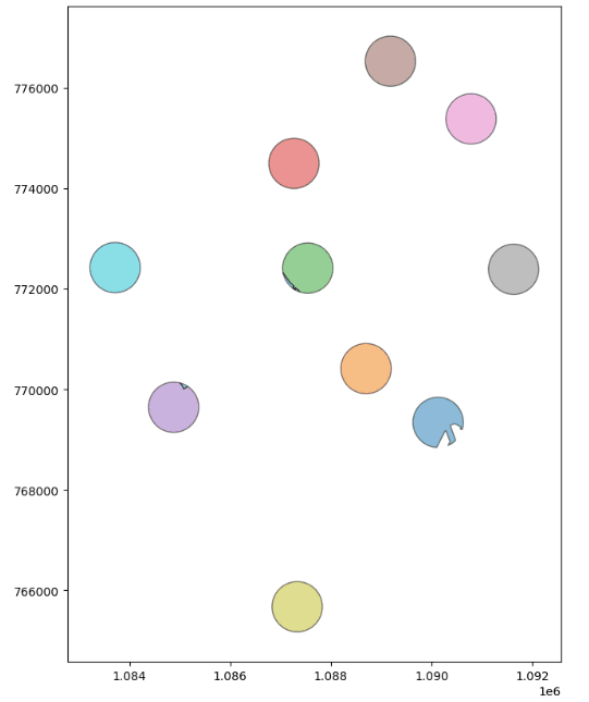
Or, if we want to see the districts without the area occupied by the projected parks, we can change the “how” parameter to perform another overlay operation.
parks_difference = districts.overlay(parks, how='difference')
ax = parks_difference.plot(alpha=0.5, edgecolor='black', column='district_name')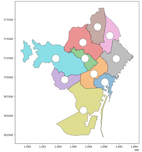
Conclusion
We hope you enjoyed this GeoPandas tutorial. Spatial analysis is one of the coolest domains in data science, providing endless opportunities to enrich your analysis with location-based information. There are many tools for spatial analysis, but if you’re already familiar with Python, GeoPandas is a great place to get started.
Willing to continue your geospatial education? We’ve got you covered! Check out our following materials and become a geospatial master:
What is geospatial data analysis?
What is GeoPandas?
What is the difference between pandas and GeoPandas?
How can I learn spatial analysis as an R programmer?
cheat sheet
Pandas Cheat Sheet for Data Science in Python

Karlijn Willems
4 min
tutorial
Introduction to Geospatial Data in Python

Duong Vu
13 min
tutorial
Python Exploratory Data Analysis Tutorial
Karlijn Willems
30 min
tutorial
Pandas Tutorial: DataFrames in Python
Karlijn Willems
20 min
tutorial
Working with Geospatial Data: A Guide to Analysis in Power BI

Joleen Bothma
10 min
tutorial
Python Seaborn Tutorial For Beginners: Start Visualizing Data

Moez Ali
20 min