Mastering Backpropagation: A Comprehensive Guide for Neural Networks

Backpropagation is an essential part of modern neural network training, enabling these sophisticated algorithms to learn from training datasets and improve over time.

Understanding and mastering the backpropagation algorithm is crucial for anyone in the field of neural networks and deep learning. This tutorial provides an in-depth exploration of backpropagation.

It starts by explaining what backpropagation is and how it works, along with its advantages and limitations, before diving into a practical experience in applying it to a widely-used dataset.

What is backpropagation?

Introduced in the 1970s, the backpropagation algorithm is the method for fine-tuning the weights of a neural network with respect to the error rate obtained in the previous iteration or epoch, and this is a standard method of training artificial neural networks.

You can think of it as a feedback system where, after each round of training or 'epoch,' the network reviews its performance on tasks. It calculates the difference between its output and the correct answer, known as the error. Then, it adjusts its internal parameters, or 'weights,' to reduce this error next time. This method is essential for tuning the neural network's accuracy and is a foundational strategy in learning to make better predictions or decisions

How Does Backpropagation Work?

Now that you know what backpropagation is, let’s dive into how it works. Below is an illustration of the backpropagation algorithm applied to a neural network of:

• Two inputs X1 and X2
• Two hidden layers N1X and N2X, where X takes the values of 1, 2 and 3
• One output layer

Backpropagation illustration (source)

There are overall four main steps in the backpropagation algorithm:

• Forward pass
• Errors calculation
• Backward pass
• Weights update

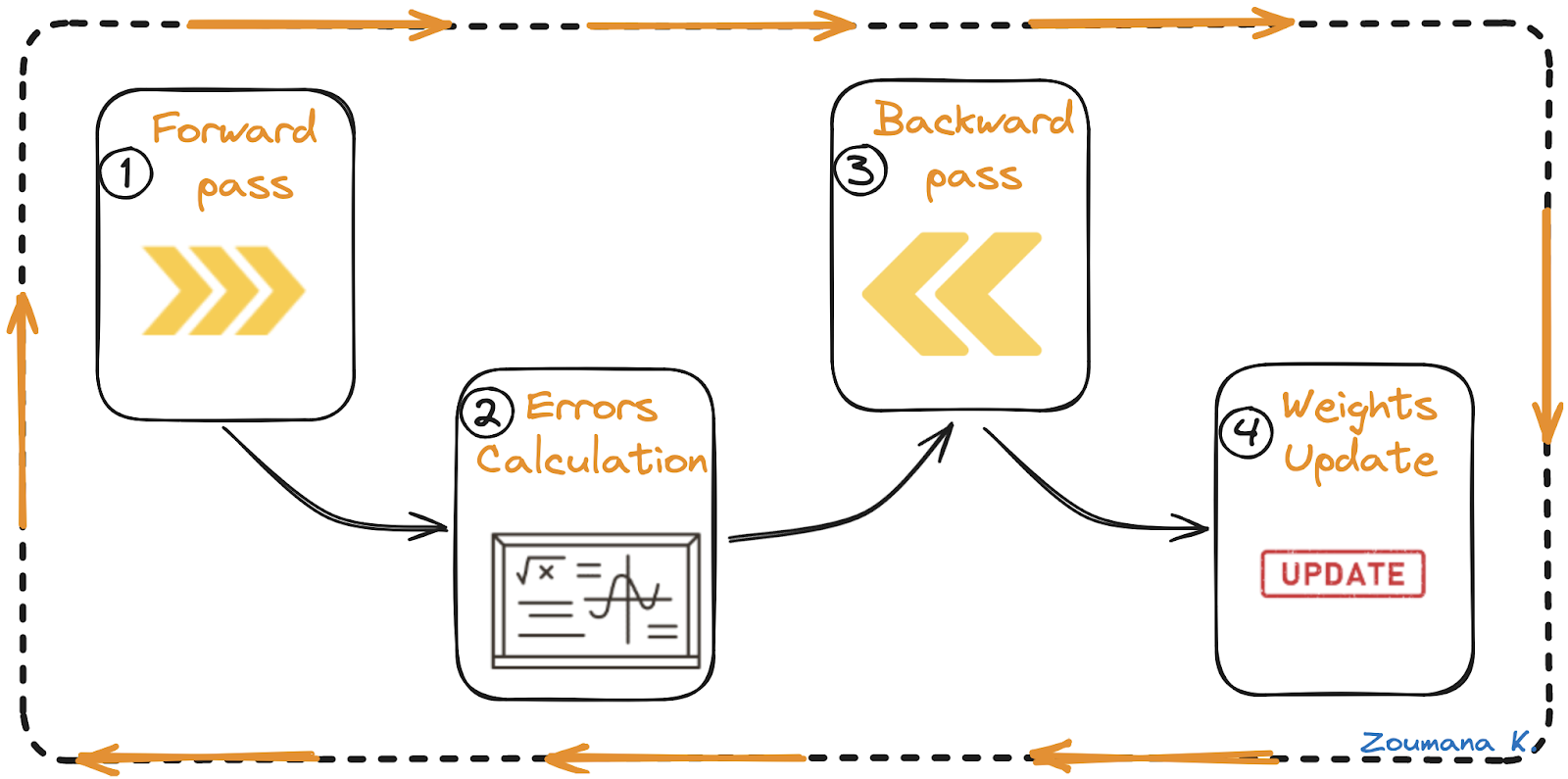
Forward pass, error calculation, backward pass, and weights update

Let’s understand each of these steps from the above animation.

Forward pass

This is the first step of the backpropagation process, and it’s illustrated below:

• The data ( inputs X1 and X2) is fed to the input layer
• Then, each input is multiplied by its corresponding weight, and the results are passed to the neurons N1X and N2X of the hidden layers.
• Those neurons apply an activation function to the weighted inputs they receive, and the result passes to the next layer.

Errors calculation

• The process continues until the output layer generates the final output (o/p).
• The output of the network is then compared to the ground truth (desired output), and the difference is calculated, resulting in an error value.

Backward pass

This is an actual backpropagation step, and can not be performed without the above forward and error calculation steps. Here is how it works:

• The error value obtained previously is used to calculate the gradient of the loss function.
• The gradient of the error is propagated back through the network, starting from the output layer to the hidden layers.
• As the error gradient propagates back, the weights (represented by the lines connecting the nodes) are updated according to their contribution to the error. This involves taking the derivative of the error with respect to each weight, which indicates how much a change in the weight would change the error.
• The learning rate determines the size of the weight updates. A smaller learning rate means than the weights are updated by a smaller amount, and vice-versa.

Weights update

• The weights are updated in the opposite direction of the gradient, leading to the name “gradient descent.” It aims to reduce the error in the next forward pass.
• This process of forward pass, error calculation, backward pass, and weights update continues for multiple epochs until the network performance reaches a satisfactory level or stops improving significantly.

Advantages of Backpropagation

Backpropagation is a foundational technique in neural network training, which is widely appreciated for its straightforward implementation, simplicity in programming, and versatile application across multiple network architectures.

Our Building Neural Network (NN) Models in R tutorial is a great starting point for anyone interested in learning about neural networks. It teaches how to create a neural network model in R.

For Python programmers, the Recurrent Neural Network Tutorial (RNN) tutorial provides a comprehensive guide about the most popular deep learning model RNN with hands-on experience by building a MasterCard stock price predictor.

Now, let’s elaborate on each of the benefits mentioned earlier:

• Ease of implementation: accessible through multiple deep learning libraries such as Pytorch and Keras, facilitating its use in diverse applications.
• Programming simplicity: simplified coding with framework abstraction, reducing the need for complex mathematics.
• Flexibility: adaptable to diverse architectures, suitable for a broad spectrum of AI challenges.

Limitations and Challenges

Despite the success of the backpropagation algorithm, it is not without limitations, which can affect the efficiency and effectiveness of the training process of a neural network. Let’s explore some of those constraints:

• Data quality: poor data quality, including noise, incompleteness, or bias, can lead to inaccurate models, as backpropagation learns exactly what it is given.
• Training duration: backpropagation often requires extensive training time, which can be impractical when dealing with large networks.
• Matrix-based complexity: the matrix operations in backpropagation scale with the network size, which increases the computational demand, and potentially outstripping the available resources.

Implementing Backpropagation

With all these insights about the backpropagation algorithm, it is time to dive into its application in a real-world scenario with the implementation of a neural network to recognize handwritten digits from the MNIST dataset.

This section covers all the steps, from data visualization to model training and evaluation. The complete source code is available in this DataLab workbook; you can easily create your own workbook copy to run the code in the browser, without installing anything on your computer.

About the dataset

The MNIST dataset is widely used in the image recognition field. It consists of 70000 grayscale images of handwritten digits from 0 to 9, and each image measures 28x28 pixels.

The dataset is available in the mnist function from the Keras.datasets module, and it is loaded as follows after importing the mnist library:

from keras.datasets import mnist
(train_images, train_labels), (test_images, test_labels) = mnist.load_data()

Exploratory data analysis

Exploratory data analysis is a major step prior to building any machine learning or deep learning model because it helps better understand the nature of the data at hand, hence, guide through the choice of the type of model to use.

The main tasks include:

• Identifying the total number of data in both training and testing dataset.
• Random visualization of some digits from the training dataset.
• Visualize the distribution of the labels from the training dataset.

The overall dataset consists of 70000 images. The typical split of the original dataset is given as follows, and there is no specific rule of thumb for that:

• 70% or 80% for the training dataset
• 30% or 20% for the testing dataset

Some split can even be 90% for training and 10% for testing.

In our scenario, the training and testing datasets are both loaded, so there is no need for splitting. Let’s observe the size of those datasets.

print("Training data")
print(f"- X = {train_images.shape}, y = {train_labels.shape}")
print(f"- Hols {train_images.shape[0]/70000* 100}% of the overall data")

print("\n")

print("Testing data")
print(f"- X = {test_images.shape}, y = {test_labels.shape}")
print(f"- Hols {test_images.shape[0]/70000* 100}% of the overall data")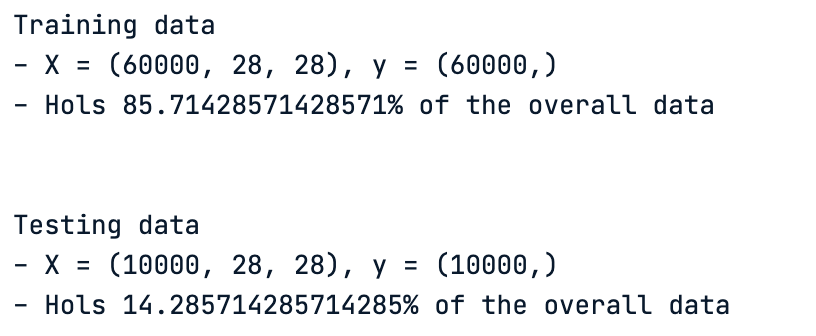

Characteristics of both training and testing datasets

• The training dataset has 60000 images and corresponds to 85.71% of the original dataset.
• The testing dataset, on the other hand, has the remaining 10000 images, hence 14.28% of the original dataset.

Now, let’s visualize some random digits. This is achieved with the helper function plot_images, which takes two main parameters:

• The number of images to plot, and
• The dataset to be considered for the visualization

def plot_images(nb_images_to_plot, train_data):

	# Generate a list of random indices from the training data
	random_indices = random.sample(range(len(train_data)), nb_images_to_plot)

	# Plot each image using the random indices
	for i, idx in enumerate(random_indices):
    	plt.subplot(330 + 1 + i)
    	plt.imshow(train_data[idx], cmap=plt.get_cmap('gray'))

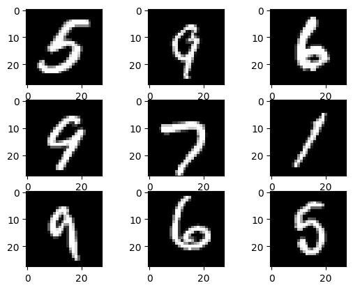
	plt.show()

We want to visualize nine images from the training data, which corresponds to the following code snippet:

nb_images_to_plot = 9
plot_images(nb_images_to_plot, train_images)

The successful execution of the above code generates the following nine digits.

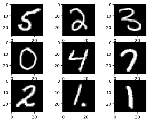
Nine random images from the training dataset

The following digits are displayed after running the same function for the second time, and we notice that they are not the same; this is due to the random nature of the helper function.

Nine random images from the training dataset after a second run of the function

The final task for the data analysis is to visualize the distribution of the labels from the training dataset using the plot_labels_distribution helper function.

• In the X-axis, we have all the possible digits
• In the Y-axis, we have the total number of such digits

import numpy as np

def plot_labels_distribution(data_labels):
    
	counts = np.bincount(data_labels)

	plt.style.use('seaborn-dark-palette')

	fig, ax = plt.subplots(figsize=(10,5))
	ax.bar(range(10), counts, width=0.8, align='center')
	ax.set(xticks=range(10), xlim=[-1, 10], title='Training data distribution')

	plt.show()

The function is applied to the training dataset by proving its labels as follows:

plot_labels_distribution(train_labels)

Below is the result, and we notice that all ten digits are almost evenly distributed across the entire dataset, which is good news, meaning that no further action is required to balance the distribution of the labels.

Data preprocessing

Real-world data usually require some preprocessing to make them suitable for training models. There are three main preprocessing tasks applied to both training and testing images:

• Image normalization: this consists of converting all the pixel values from 0-255 to 0-1. This is relevant for a faster convergence during the training process
• Reshaping images: instead of having a squared matrix of 28 by 28 for each image, we flatten each one into 784-element vectors in order to make it suitable for the neural network inputs.
• Label encoding: convert the labels to one-hot encoded vectors. This will avoid the issues we might have with the numerical hierarchy. This way, the model will be biased towards larger digits.

The overall preprocessing logic is implemented in the helper function preprocess_data below:

from keras.utils import to_categorical

def preprocess_data(data, label,
                	vector_size,
                	grayscale_size):
    
	# Normalize to range 0-1
	preprocessed_images = data.reshape((data.shape[0],
                             	vector_size)).astype('float32') / grayscale_size
    
	# One-hot encode the labels
	encoded_labels = to_categorical(label)
    
	return preprocessed_images, encoded_labels

The function is applied to the datasets using these code snippets:

# Flattening variable
vector_size = 28 * 28

grayscale_size = 255
train_size = train_images.shape[0]
test_size = test_images.shape[0]

# Preprocessing of the training data
train_images, train_labels = preprocess_data(train_images,
                                         	train_labels,
                                         	vector_size,
                                         	grayscale_size)

# Preprocessing of the testing data
test_images, test_labels = preprocess_data(test_images,
                                       	test_labels,
                                       	vector_size,
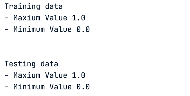
                                       	grayscale_size)

Now, let’s observe the current maximum and minimum pixel values of both datasets:

print("Training data")
print(f"- Maxium Value {train_images.max()} ")
print(f"- Minimum Value {train_images.min()} ")

print("\n")

print("Testing data")
print(f"- Maxium Value {test_images.max()} ")
print(f"- Minimum Value {test_images.min()} ")

The result of the code is given below, and we notice that the normalization was successfully performed.

Minimum and maximum pixel values after normalization

Similarly to the labels, we finally have a matrix of ones and zeros, which correspond to the one-hot encoded values of those labels.

# One hot encoding of the test data labels
test_images

Result below:

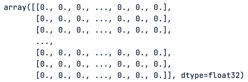
One hot encoding of the test data labels

# One hot encoding of the train data labels
train_labels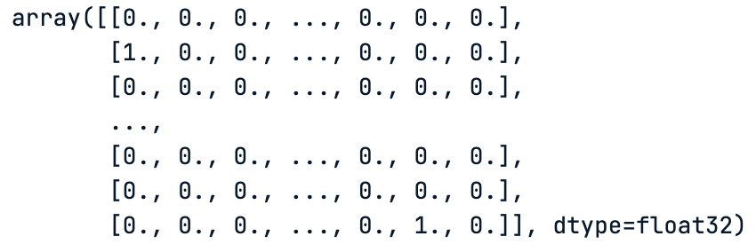

One hot encoding of the train data labels

Structure of the network

Since we are using an image classification task, a convolution neural network is more adapted for such a scenario. Before coding anything, it is important to define the architecture of the model, and that is the whole point of this section.

To learn more about convolutional neural networks, our An Introduction to Convolutional Neural Networks (CNNs) tutorial is a great starting resource. It is a complete guide to understanding CNNs, their impact on image analysis, and some key strategies to combat overfitting for robust CNN vs deep learning applications.

The architecture for this use case combines different types of layers for an effective image classification. Below are the key components of the model:

• Convolutional Layer: Begin with a layer using a small 3x3 filter size and 32 filters to process the images.
• Max Pooling Layer: After the convolutional layer, include a max pooling layer to reduce the size of the feature maps.
• Flattening: Flatten the output of the pooling layer into a single vector, preparing it for the classification process.
• Dense Layer: Add a dense layer with 100 nodes between the flattened output and the final layer to interpret the extracted features.
• Output Layer: Use an output layer with 10 nodes, corresponding to the 10 image categories. Each node calculates the probability of an image belonging to one of these categories.
• Softmax Activation: In the output layer, apply a softmax activation function for multi-class classification.
• ReLU Activation Function: Utilize the ReLU (Rectified Linear Unit) activation function in all layers for non-linear processing.
• Optimizer: Employ a stochastic gradient descent optimizer with a learning rate of 0.001 and momentum of 0.95 for adjusting the model during training.
• Loss Function: Use the categorical cross-entropy loss function, ideal for multi-class classification tasks.
• Accuracy Metric: Focus on the classification accuracy metric, considering the balanced distribution of classes.

All this information is implemented in the define_network_architecture helper function. But before that, we need to import all the necessary libraries:

from keras import models
from keras import layers
from tensorflow.keras.optimizers import SGD
from tensorflow.keras.layers import Conv2D
from tensorflow.keras.models import Sequential
from tensorflow.keras.layers import MaxPooling2D
from tensorflow.keras.layers import Dense
from tensorflow.keras.layers import Flatten
from tensorflow.keras.layers import BatchNormalization 

Here is the implementation of the helper function.

hidden_units = 256
nb_unique_labels = 10
vector_size = 784  # Assuming a 28x28 input image for example

def define_network_architecture():

	network = models.Sequential()
	network.add(Dense(vector_size, activation='relu', input_shape=(vector_size,)))  # Input layer
	network.add(Dense(512, activation='relu'))                       	# Hidden layer
	network.add(Dense(nb_unique_labels, activation='softmax'))  

	return network

The source code implementation is good, but it is even better if we can have a graphical visualization of the network, and this is achieved using the plot_model function from the keras.utils.vis_utils module.

First, generate the network from the helper function.

network = define_network_architecture()

Then, display the graphical representation. We first save the result into a PNG file before showing it; this makes it easier to share with others.

import keras.utils.vis_utils
from importlib import reload
reload(keras.utils.vis_utils)
from keras.utils.vis_utils import plot_model    

import matplotlib.image as mpimg

plot_model(network, to_file='network_architecture.png', show_shapes=True, show_layer_names=True)

img = mpimg.imread('network_architecture.png')
plt.imshow(img)
plt.axis('off')
plt.show()

The result is shown below.

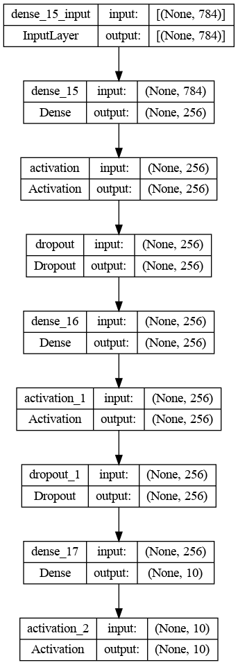
Graphical architecture of the convolutional neural network

Calculating the delta

Before diving into the training process of the model, let’s understand how the delta error distribution is calculated using the architecture of the network.

The delta error distribution is the derivative of the loss function with respect to the activation function of each node, and it indicates how much each node’s activation contributed to the final error.

The above architecture consists of three main layers:

• Input layer of 784 unites corresponding to a 28x28 input image
• Hidden layer of 512 unites with the ReLU activation
• Output layer with 10 units, which correspond to the number of unique labels with softmax activation function

Now, let’s go further with the delta error calculation for each layer.

Output layer

Let’s consider the output of the softmax layer as big O (O) and the true labels as Y. By using the cross-entropy loss δ output , the delta error becomes:

δ output = O - Y

This formula comes from the basic calculation of how the cross-entropy loss changes when the softmax output changes.

Hidden layer

For the hidden layer, the delta error becomes δ hidden and depends on the error of the subsequent layer, which corresponds to the output layer, and the derivative of the activation ReLU function.

The derivative of the ReLU is 1 for positive inputs, and 0 for negative ones, as shown below.

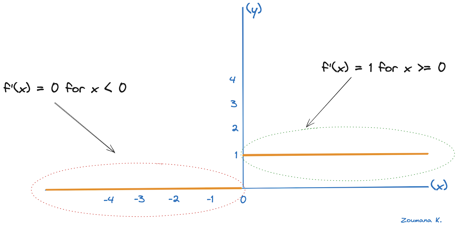
Derivative illustration of the ReLU

Let’s consider Zhidden to be the input to the ReLU function in the hidden layer and Woutput to be the weights connecting the hidden layer to the output layer. The delta error for the hidden layer, in this case, becomes:

δ hidden = (δ output . Woutput) ⊙ ReLU’(Zhidden)

• The dot sign “.” denotes the matrix multiplication
• The sign ⊙ corresponds to element-wise multiplication
• ReLU’(Zhidden) Corresponds to the derivative of the ReLU at Zhidden

Input layer

Similarly, if we had more hidden layers, the process would continue backwards with each layer’s delta error depending on the subsequent layer’s delta error and the derivative of its activation function.

In a more general scenario, for any given layer k in the network (except the output layer), the formula for delta error calculation is:

δ _k = (δ _k+1 . W^T_k+1) ⊙ f’(Z_k)

• W^T_k+1 corresponds to the transpose of the weights matrix of the next layer
• f’ is the derivative of the activation function for layer k and
• Z_k is the input to the activation function in layer k

Compilation of the network

With this understanding of the error computation, let’s compile the network to optimize its structure for the training process.

During compilation, we need to make several critical choices:

• Choice of Optimization Algorithm: this involves selecting an algorithm for gradient descent optimization. There are multiple options, such as Stochastic Gradient Descent (SGD), Adagrad, and RMSprop, which is used in this article.
• Selection of a Loss Function: The loss function, also known as the cost function, is an essential part of training. It quantifies how well the network performs, and the choice of loss function should align with the nature of the classification or regression problem. The focus is made on the categorical cross entropy because of multi-class nature of the problem.
• Choice of a Performance Metric: While similar to a loss function, a performance metric is primarily used to evaluate the model's effectiveness on the test dataset, and we are using the accuracy

The code for the above three choices is given below:

network.compile(optimizer='rmsprop',
            	loss='categorical_crossentropy',
            	metrics=['accuracy'])

Training of the network

One of the biggest issues for training a model is overfitting, and it is crucial to monitor the model during the training process to ensure that it has a better generalization, and one way of doing that is the concept of early stopping.

The complete logic is illustrated below:

# Fit the model
batch_size = 256
n_epochs = 15
val_split = 0.2
patience_value = 5

# Fit the model with the callback
history = network.fit(train_images, train_labels, validation_split=val_split,
        	epochs=n_epochs, batch_size=batch_size)

The model is trained for 15 epochs using a batch size of 256, and 20% of the training data is used for validation of the model.

After training the model, the training and validation performance history is plotted below.

plt.plot(history.history['accuracy'])
plt.plot(history.history['val_accuracy'])
plt.title('Model accuracy')
plt.ylabel('Accuracy')
plt.xlabel('Epoch')
plt.legend(['Train', 'Validation'], loc='upper left')
plt.show()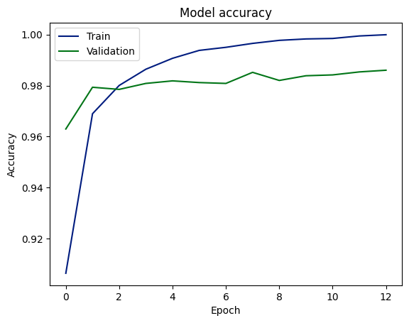

​​

Training and validation accuracy scores

Evaluation on test data

Now, we can evaluate the model performance on the test data using the evaluate function of the model.

loss, acc = network.evaluate(test_images,
                         	test_labels, batch_size=batch_size)

print("\nTest accuracy: %.1f%%" % (100.0 * acc))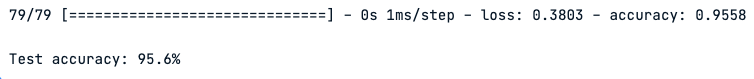

Model performance on test data

The graph indicates that the model has learned to predict outcomes with high accuracy, achieving around 98% on both validation and test data sets. This suggests good generalization from training to unseen data. However, the gap between training and validation accuracy could be a sign of overfitting, although the consistency between validation and test accuracy might mitigate this concern.

Recommendation

Even though the model shows high accuracy and generalization capabilities, there is still room for improvement, and below are some actionable steps to further improve the performance.

• Regularization: Integrate regularization methods to reduce overfitting.
• Early Stopping: Utilize early stopping during training to prevent overfitting.
• Error Analysis: Analyze mispredictions to identify and correct underlying issues.
• Diversity Testing: Test the model on varied datasets to confirm its robustness.
• Broader Metrics: Use precision, recall, and F1-score for a complete performance evaluation, especially if data is imbalanced.

Conclusion

In summary, this article has provided a comprehensive exploration of backpropagation, an essential technique in the field of machine learning. We started with a clear definition of what backpropagation is and outlined its critical role in the advancement of artificial intelligence.

Next, we dived into the workings of backpropagation along with some of its advantages, such as improved learning efficiency, while also acknowledging the limitations and challenges it faces.

Then, it provided detailed guidance on setting up and building neural networks, emphasizing the significance of forward propagation.

In the concluding sections, we explored steps of calculating deltas and updating network weights, which are essential for refining the learning process.

Overall, this article serves as a valuable resource for anyone aiming to understand and effectively implement backpropagation in neural networks.

Are you eager to strengthen your skills in deep learning? Our Deep Learning with PyTorch course will help you acquire the confidence to delve deeper into neural networks and progress your knowledge further.