How to Execute SQL Queries in Python and R Tutorial

Creating a Database

In this part, we will learn how to load the COVID-19's impact on airport traffic dataset, under the CC BY-NC-SA 4.0 license, into our SQLite database. We will also learn how to create tables from scratch.

The airport traffic dataset consists of a percentage of the traffic volume during the baseline period from February 1, 2020, to March 15, 2020. We will load a CSV file by using Pandas function read_csv and then use the to_sql function to transfer the dataframe into our SQLite table. The to_sql function requires a table name (String) and connection to the SQLite engine.

data = pd.read_csv("data/covid_impact_on_airport_traffic.csv")


data.to_sql(
            'airport',             # Name of the sql table
            conn,                 # sqlite.Connection or sqlalchemy.engine.Engine
            if_exists='replace'
           )

We will now test whether we have succeeded by running a quick SQL query. Before running a query, we need to create a cursor that will help us execute queries, as shown in the code block below. You can have multiple cursors on the same database within a single connection.

In our case, the SQL query returned three columns and five rows from the airport table. To display the first row, we will use cursor.fetchone().

cursor = conn.cursor()
cursor.execute("""SELECT Date, AirportName, PercentOfBaseline  
                  FROM airport
                  LIMIT 5""")
cursor.fetchone()


>>> ('2020-04-03', 'Kingsford Smith', 64)

To display the rest of the records, we will use cursor.fetchall(). The airport dataset is successfully loaded into the database with a few lines of code.

cursor.fetchall()

>>> [('2020-04-13', 'Kingsford Smith', 29),
     ('2020-07-10', 'Kingsford Smith', 54),
     ('2020-09-02', 'Kingsford Smith', 18),
     ('2020-10-31', 'Kingsford Smith', 22)]

Now, let’s learn to create a table from scratch and populate it by adding sample values. We will create a studentinfo table with id (integer, primary key, auto-increment), name (text), and subject (text).

Note: The SQLite syntax is a bit different. It is recommended to check out the SQLite cheat sheet to understand the SQL queries mentioned in this tutorial.

cursor.execute("""
                CREATE TABLE studentinfo
                (
                id INTEGER PRIMARY KEY AUTOINCREMENT,
                name TEXT,
                subject TEXT
                )
                 """)

Let’s check how many tables we have added to the database by running a simple SQLite query.

cursor.execute("""
                SELECT name
                FROM sqlite_master
                WHERE type='table'
                 """)
cursor.fetchall()

>>> [('airport',), ('studentinfo',)]

Running Queries

In this section, we will add values to the studentinfo table and run simple SQL queries. By using INSERT INTO, we can add a single row to the studentinfo table.

To insert values, we need to provide a query and value arguments to the execute function. The function fills the “?” inputs with the values that we have provided.

query = """
            INSERT INTO studentinfo
            (name, subject)
            VALUES (?, ?)
        """
value = ("Marry", "Math")
cursor.execute(query,value)

Repeat the above query by adding multiple records.

query = """
           INSERT INTO studentinfo
           (name, subject)
           VALUES (?, ?)
        """
values = [("Abid", "Stat"),
          ("Carry", "Math"),
          ("Ali","Data Science"),
          ("Nisha","Data Science"),
          ("Matthew","Math"),
          ("Henry","Data Science")]

cursor.executemany(query,values)

It’s time to verify the record. To do this we will run a simple SQL query that will return rows where the subject is Data Science.

cursor.execute("""
                SELECT *
                FROM studentinfo
                WHERE subject LIKE 'Data Science'
                 """)
cursor.fetchall()

>>> [(4, 'Ali', 'Data Science'),
     (5, 'Nisha', 'Data Science'),
     (7, 'Henry', 'Data Science')]

The DISTINCT subject command is used to display unique values present in subject columns. In our case, it’s Math, Stat, and Data Science.

cursor.execute("SELECT DISTINCT subject from studentinfo")
cursor.fetchall()

>>> [('Math',), ('Stat',), ('Data Science',)]

To save all of the changes, we will use the commit() function. Without a commit, the data will be lost after the machine restarts.

conn.commit()

SQL with Pandas

In this part we will learn how to extract the data from the SQLite database and convert it into a Pandas dataframe with one line of code. read_sql provides more than just running SQL queries. We can use it for setting index columns, parsing date and time, adding values, and filtering out column names. Learn more about importing data in Python by taking a short DataCamp course.

read_sql requires two arguments: a SQL query and connection to the SQLite engine. The output contains the top five rows from the airport table where PercentOfBaseline is greater than 20.

data_sql_1 = pd.read_sql("""
                        SELECT Date,City,PercentOfBaseline
                        FROM airport
                        WHERE PercentOfBaseline > 20
                        ORDER BY Date DESC
                        """,
                        conn)
print(data_sql_1.head())

         Date          City  PercentOfBaseline
0  2020-12-02        Sydney                 27
1  2020-12-02      Santiago                 48
2  2020-12-02       Calgary                 99
3  2020-12-02  Leduc County                100
4  2020-12-02      Richmond                 86

Running data analysis on relational databases has become easier with Pandas integration. We can also use this data to forecast the values and run complex statistical analyses.

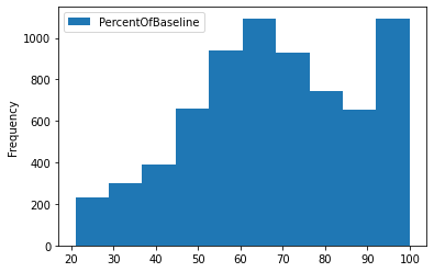
The plot function is used to visualize the histogram of the PercentOfBaseline column.

data_sql_1.plot(y="PercentOfBaseline",kind="hist");

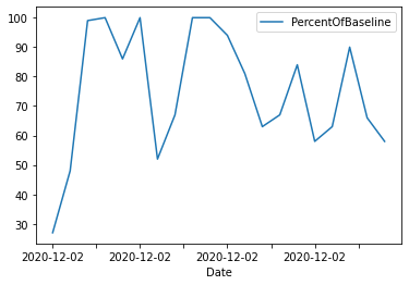
Similarly, we can limit the values to the top 20 and display a time series line chart.

data_sql_2 = pd.read_sql("""
                        SELECT Date,City,PercentOfBaseline
                        FROM airport
                        WHERE PercentOfBaseline > 20
                        ORDER BY Date DESC
                        LIMIT 20
                        """,
                        conn)


data_sql_2.plot(x="Date",y="PercentOfBaseline",kind="line");

Finally, we will close the connection to free up resources. Most packages do this automatically, but it is preferred to close the connections after finalizing the changes.

conn.close()

R Tutorial

We are going to replicate all the tasks from the Python tutorial using R. The tutorial includes creating connections, writing tables, appending rows, running queries, and data analysis with dplyr.

Setting Up

The DBI package is used for connecting with the most popular databases such as MariaDB, Postgres, Duckdb, and SQLite. For example, install the RMySQL package and create a database by providing a username, password, database name, and host address.

install.packages("RMySQL")
library(RMySQL)
conn = dbConnect(
                MySQL(),
                user = 'abid',
                password = '1234',
                dbname = 'datacamp_R',
                host = 'localhost'
                )

In this tutorial, we are going to create an SQLite database by providing a name and the SQLite function.

library(RSQLite)
library(DBI)
library(tidyverse)

conn = dbConnect(SQLite(), dbname = 'datacamp_R.db')

Creating Database

By importing the tidyverse library, we will have access to the dplyr, ggplot, and defaults datasets.

dbWriteTable function takes data.frame and adds it into the SQL table. It takes three arguments: connection to SQLite, name of the table, and data frame. With dbReadTable, we can view the entire table. To view the top 6 rows, we have used head.

dbWriteTable(conn, "cars", mtcars)
head(dbReadTable(conn, "cars"))

    mpg    cyl    disp    hp    drat    wt    qsec    vs    am    gear    carb
1    21.0    6    160    110    3.90    2.620    16.46    0    1    4    4
2    21.0    6    160    110    3.90    2.875    17.02    0    1    4    4
3    22.8    4    108    93    3.85    2.320    18.61    1    1    4    1
4    21.4    6    258    110    3.08    3.215    19.44    1    0    3    1
5    18.7    8    360    175    3.15    3.440    17.02    0    0    3    2
6    18.1    6    225    105    2.76    3.460    20.22    1    0    3    1

dbExecute lets us execute any SQLite query, so we will be using it to create a table called idcard.

To display the names of the tables in the database, we will use dbListTables.

dbExecute(conn, 'CREATE TABLE idcard (id int, name text)')
dbListTables(conn)

>>> 'cars''idcard'

Let’s add a single row to the idcard table and use dbGetQuery to display results.

Note: dbGetQuery runs a query and returns the records whereas dbExecute runs SQL query but does not return any records.

dbExecute(conn, "INSERT INTO idcard (id,name)\
                 VALUES(1,'love')")
dbGetQuery(conn,"SELECT * FROM idcard")


id    name
1    love

We will now add two more rows and display results by using dbReadTable.

dbExecute(conn,"INSERT INTO idcard (id,name)\
                VALUES(2,'Kill'),(3,'Game')
               ")
dbReadTable(conn,'idcard')


id    name
1    love
2    Kill
3    Game

dbCreateTable lets us create a hassle-free table. It requires three arguments; connection, name of the table, and either a character vector or a data.frame. The character vector consists of names (column names) and values (types). In our case, we are going to provide a default population data.frame to create the initial structure.

dbCreateTable(conn,'population',population)
dbReadTable(conn,'population')

country    year    population

Then, we are going to use dbAppendTable to add values in the population table.

dbAppendTable(conn,'population',head(population))
dbReadTable(conn,'population')

country    year    population
Afghanistan    1995    17586073
Afghanistan    1996    18415307
Afghanistan    1997    19021226
Afghanistan    1998    19496836
Afghanistan    1999    19987071
Afghanistan    2000    20595360

Running Queries

We will use dbGetQuery to perform all of our data analytics tasks. Let’s try to run a simple query and then learn more about other functions.

dbGetQuery(conn,"SELECT * FROM idcard")

id    name
1    love
2    Kill
3    Game

You can also run a complex SQL query to filter horsepower and display limited rows and columns.

dbGetQuery(conn, "SELECT mpg,hp,gear\
                  FROM cars\
                  WHERE hp > 50\
                  LIMIT 5")


mpg    hp    gear
21.0    110    4
21.0    110    4
22.8    93    4
21.4    110    3
18.7    175    3

To remove tables, use dbRemoveTable. As we can now see, we have successfully removed the idcard table.

dbRemoveTable(conn,'idcard')
dbListTables(conn)
>>> 'cars''population'

To understand more about tables we will use dbListFields which will display the column names in a particular table.

dbListFields(conn, "cars")


>>> 'mpg''cyl''disp''hp''drat''wt''qsec''vs''am''gear''carb'

SQL with dplyr

In this section, we will use dplyr to read tables and then run queries using filter, select, and collect. If you don’t want to learn SQL syntax and want to perform all the tasks using pure R, then this method is for you. We have pulled the cars table, filtered it by gears and mpg, and then selected three columns as shown below.

cars_results <-
  tbl(conn, "cars") %>%
  filter(gear %in% c(4, 3),
         mpg >= 14,
         mpg <= 21) %>%
  select(mpg, hp, gear) %>%
  collect()
cars_results

mpg    hp    gear
21.0    110    4
21.0    110    4
18.7    175    3
18.1    105    3
14.3    245    3
...   ...   ...

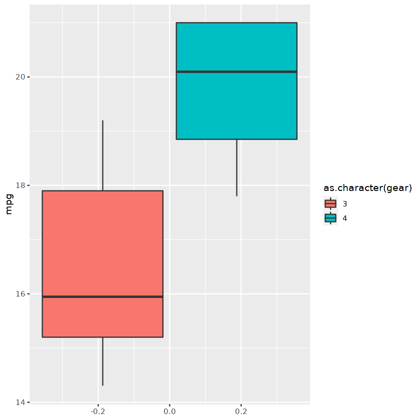
We can use the filtered data frame to display a boxplot graph using ggplot.

ggplot(cars_results,aes(fill=as.character(gear), y=mpg)) +
  geom_boxplot()

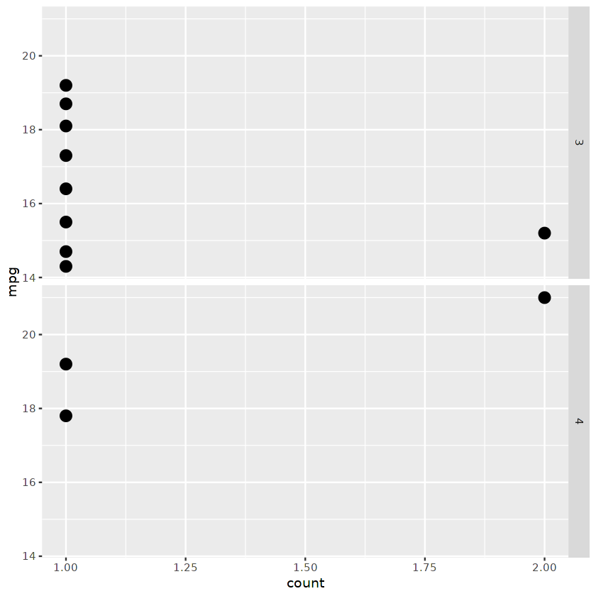
Or we can display a facet point plot divided by the number of gears.

ggplot(cars_results,
  aes(mpg, ..count.. ) ) +
  geom_point(stat = "count", size = 4) +
  coord_flip()+
  facet_grid( as.character(gear) ~ . )

Conclusion

In this tutorial, we have learned the importance of running SQL queries with Python and R, creating databases, adding tables, and performing data analysis using SQL queries. We have also learned how Pandas and dplyr help us run queries with a single line of code.

SQL is a must-learn skill for all tech-related jobs. If you are starting your career as a data analyst, we recommend completing the Data Analyst with SQL Server career track within two months. This career track will teach you everything about SQL queries, servers, and managing resources.

You can run all the scripts used in this tutorial for free by clicking on the green button Open In Workspace.

• The SQL with Python project is available on the DataCamp Python workspace.
• The SQL with R project is available on the DataCamp R workspace.