Batch Normalization: Theory and TensorFlow Implementation

Training deep neural networks can be challenging due to vanishing or exploding gradients and internal covariate shift. These factors can significantly slow down the training process and hinder the network's ability to learn effectively. Fortunately, we can address these issues with normalization techniques.

While there are many normalization techniques, batch normalization is one of the most popular and has become a standard component in many deep learning architectures. It contributes to faster convergence, improved training stability, and better generalization performance.

In this tutorial, we’ll explain batch normalization, how it works mathematically, and how to implement it using TensorFlow and Keras.

If you want to learn the fundamentals of neural networks using Keras, check out this Introduction to Deep Learning in Python course.

What is Normalization in Machine Learning?

Normalization is a crucial preprocessing step in machine learning that aims to standardize the input data.

Various normalization techniques, such as min-max scaling, z-score normalization, and log transformation, are commonly used to rescale features to a consistent range or distribution. These techniques help mitigate the impact of outliers, improve convergence, and ensure a fair comparison between features.

Normalizing input data is essential for effective model training because it ensures that all features contribute equally to the learning process. Without normalization, features with larger scales or variances can dominate the optimization process, leading to suboptimal model performance.

Normalization allows the model to learn meaningful patterns and relationships from the data by bringing all features to a similar scale.

If you want to learn about normalization in general, check out this tutorial on What is Normalization in Machine Learning.

Deep Learning Training Challenges

Training deep neural networks presents several challenges that can hinder convergence and generalization:

1. Internal covariate shift: As the input data passes through multiple layers, the distribution of activations can change, making it difficult for the model to adapt and learn effectively.
2. Vanishing and exploding gradients: Deep networks can suffer from vanishing or exploding gradients, where the gradients become too small or too large during backpropagation, preventing effective weight updates.
3. Sensitivity to initialization: The initial weights of the network can significantly impact the training process, and poor initialization can lead to slow convergence or even training failure.

Batch normalization addresses these challenges by normalizing the activations within each mini-batch, helping to stabilize the training process and improve the model's performance.

What is Batch Normalization?

Batch normalization is a technique that normalizes the activations of a layer within a mini-batch during the training of deep neural networks.

It operates by calculating the mean and variance of the activations for each feature in the mini-batch and then normalizing the activations using these statistics.

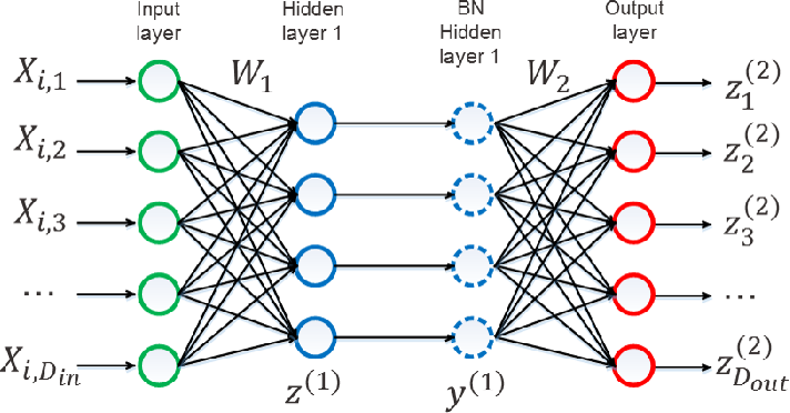
The normalized activations are then scaled and shifted using learnable parameters, allowing the model to adapt to the optimal activation distribution.

Source: Yintai Ma and Diego Klabjan.

Batch Normalization is typically applied after the linear transformation of a layer (e.g., after the matrix multiplication in a fully connected layer or after the convolution operation in a convolutional layer) and before the non-linear activation function (e.g., ReLU).

The key components of batch normalization are:

1. Mini-batch statistics: The mean and variance of the activations are calculated for each feature within the mini-batch.
2. Normalization: The activations are normalized by subtracting the mini-batch mean and dividing by the mini-batch standard deviation.
3. Scaling and shifting: Learnable parameters (γ and β) are introduced to scale and shift the normalized activations, allowing the model to learn the optimal activation distribution.

Why Use Batch Normalization?

One of the challenges we face when training deep neural networks is the internal covariate shift. This happens when the distribution of activations (outputs) from one layer changes throughout the training process as weights in previous layers are updated. This shift can make training difficult and slow.

Batch normalization reduces this shift by normalizing the activations within each mini-batch, making the inputs to subsequent layers more stable and consistent.

Normalizing activations allows for faster convergence with higher learning rates and makes the model less sensitive to initialization choices.

Additionally, it introduces a regularizing effect that helps prevent overfitting by reducing the model's dependence on specific activation patterns.

This combination of benefits makes batch normalization a powerful tool for training more robust deep learning models. To learn more about building robust models, check out this course on Machine Learning Monitoring Concepts.

The Mathematics Behind Batch Normalization

Now that we understand the “why” behind batch normalization, let’s delve into the “how.”

Batch normalization operates differently during training and inference stages, so let’s explain the mathematics behind each stage.

Batch normalization during training

Let’s start with the normalization step. We first calculate the mean and variance for each feature in a mini-batch. These are the formulas we can use for the mean and the variance.

We then use the mean and variance to normalize the activations. This is the formula we can use, where the ε (lowercase epsilon) is a small constant added for numerical stability:

After we’re done with the normalization step, we move on to the scaling and shifting step. Using the learnable parameters γ and β, we shift the normalized activations using this formula:

These parameters allow the model to learn the optimal activation distribution.

Batch normalization during inference

During inference, we replace the batch statistics (mean and variance) with the running statistics computed during training. The running statistics are typically updated using a moving average with a momentum factor.

To calculate the running mean and variance, we can use these two formulas, where α is the momentum factor that controls the update rate of the running statistics:

The running mean and variance are stored as model parameters and used for normalization during inference. The scaling and shifting parameters (γ and β) learned during training are also used during inference.

Next, let’s learn how to implement batch normalization using TensorFlow.

Batch Normalization in TensorFlow

Let’s start by importing the necessary libraries:

import tensorflow as tf 
from tensorflow import keras

Next, let’s load the MNIST dataset, which consists of 60,000 training images and 10,000 test images of handwritten digits. We load the dataset using the keras.datasets.mnist.load_data() function and split it into training data (x_train, y_train) and test data (x_test, y_test):

# Load the MNIST dataset
(x_train, y_train), (x_test, y_test) = keras.datasets.mnist.load_data()

To preprocess the data, we take the following steps:

• We reshape the training and test images to have a shape of (num_samples, 28, 28, 1), where num_samples is the number of images, and each image is a 28x28 grayscale image with a single channel.
• We normalize the pixel values of the images by dividing them by 255.0 to scale them between 0 and 1.
• We convert the training and test labels to a categorical format using keras.utils.to_categorical(), which converts the integer labels to one-hot encoded vectors.

# Preprocess the data
x_train = x_train.reshape((60000, 28, 28, 1)) / 255.0  # Reshape and normalize training images
x_test = x_test.reshape((10000, 28, 28, 1)) / 255.0    # Reshape and normalize test images
y_train = keras.utils.to_categorical(y_train)         # Convert training labels to categorical format
y_test = keras.utils.to_categorical(y_test)           # Convert test labels to categorical format

Now, we move on to the next step: defining the model architecture. To do that, we take the following steps:

• We define the model architecture using the keras.Sequential API, which allows stacking layers sequentially.
• The model consists of convolutional layers (Conv2D) for feature extraction, followed by batch normalization layers (BatchNormalization) to normalize the activations.
• We use max pooling (MaxPooling2D) for downsampling the feature maps.
• We flatten the feature maps (Flatten) before passing them to the dense layers.
• The final dense layer has 10 units with softmax activation, corresponding to the 10 classes of digits.

# Define the model architecture
model = keras.Sequential([
    keras.layers.Conv2D(32, (3, 3), activation='relu', input_shape=(28, 28, 1)),
    keras.layers.BatchNormalization(),
    keras.layers.Conv2D(64, (3, 3), activation='relu'),
    keras.layers.BatchNormalization(),
    keras.layers.MaxPooling2D((2, 2)),
    keras.layers.Flatten(),
    keras.layers.Dense(128, activation='relu'),
    keras.layers.BatchNormalization(),
    keras.layers.Dense(10, activation='softmax')
])

• The Adam optimizer ('adam') for optimization.
• The categorical cross-entropy loss ('categorical_crossentropy') as the loss function since the problem is a multi-class classification task.
• Accuracy ('accuracy') as the evaluation metric to measure the model's performance.

# Compile the model
model.compile(optimizer='adam',
              loss='categorical_crossentropy',
              metrics=['accuracy'])

Next, let’s train the mode using the .fit() method:

• We specify the training data (x_train, y_train), batch size, number of epochs, and validation data (x_test, y_test).
• The batch_size determines the number of samples per gradient update.
• The epochs parameter specifies the number of times the model will iterate over the entire training data.
• The validation data is used to evaluate the model's performance on unseen data during training.

# Train the model
model.fit(x_train, y_train, batch_size=128, epochs=5, validation_data=(x_test, y_test))

By following these steps and incorporating batch normalization layers into the model architecture, we can train the model efficiently on the MNIST dataset, benefiting from the normalization of activations and improved training stability.

Now that we have learned about batch normalization and how to implement it, let’s examine its benefits.

Implementation Considerations

Let’s now take a deeper look at implementing batch normalization in deep learning architectures.

Placement in neural network architectures

Batch normalization layers are most effective when placed strategically within our network. Typically, they are placed after the linear transformation (e.g., convolutional or fully connected layers) and before the non-linear activation function.

In convolutional networks, this translates to placing batch normalization after each convolutional layer and before the activation function.

Similarly, in fully connected networks, it's common to add batch normalization after the linear transformation and before the activation function of each hidden layer.

The placement of batch Normalization layers can influence our model's performance and training dynamics. Experimentation might be necessary to find the optimal configuration for each specific network architecture.

Impact of batch size

The batch size used during training can affect the effectiveness of batch normalization. Larger batch sizes provide more accurate estimates of the batch statistics (mean and variance), leading to better normalization and more stable training.

However, increasing the batch size also increases memory consumption and computational requirements, which may be a constraint depending on the available hardware resources.

It's important to balance batch size and computational feasibility while ensuring that the batch statistics remain reliable for normalization.

Regularization effects and implications

Batch normalization inherently introduces a regularization effect due to the noise induced by the mini-batch statistics. The stochasticity introduced by the batch statistics acts as a form of regularization, reducing overfitting and improving generalization.

However, this regularization effect may interact with other regularization techniques, such as dropout or L2 regularization.

When using batch normalization, it's essential to consider the interplay between different regularization methods and adjust them accordingly to avoid over-regularization or diminished performance.

Experimentation and monitoring the model's performance on validation data can help find the right balance of regularization techniques when using batch normalization.

Limitations and Challenges of Batch Normalization

While batch normalization is a useful technique, there are a few limitations and challenges that we need to be aware of.

Batch normalization in non-convolutional architectures

Batch Normalization was originally designed for convolutional neural networks (CNNs) and has been particularly successful in this domain.

However, its effectiveness in non-convolutional architectures, such as recurrent neural networks (RNNs) or transformers, may be limited.

The sequential nature of RNNs and the attention mechanisms in transformers can make applying batch normalization more challenging.

Alternative normalization techniques, such as layer normalization or instance normalization, may be more suitable for these architectures.

Small batch sizes and inference-time performance

Batch normalization relies on the batch statistics computed during training to normalize the activations. When the batch size is small, the batch statistics may become less reliable and introduce noise or instability in the normalization process.

This can lead to suboptimal performance or even training difficulties, especially when the batch size is reduced to accommodate memory constraints.

During inference, batch normalization uses the running statistics computed during training, which may not accurately represent the statistics of individual samples or small batches. This can result in a mismatch between the training and inference distributions, potentially impacting the model's performance.

Drawbacks and trade-offs of batch normalization

Batch normalization introduces additional computational overhead during training due to the calculation of batch statistics and the normalization operation. This overhead can increase the memory requirements and training time, especially for large models or datasets.

Batch normalization may be unsuitable for certain types of data or tasks where the normalization process can distort important information or remove meaningful variations.

For example, batch normalization may have undesirable effects on tasks involving fine-grained details or precise spatial information, such as segmentation or localization.

The regularization effect of Batch Normalization can sometimes interact with other regularization techniques, such as dropout, in unexpected ways, requiring careful tuning and consideration.

How to Mitigate the Limitations of Batch Normalization

Despite limitations and challenges, batch normalization remains a widely used and effective technique in deep learning. Researchers and practitioners continue exploring ways to address these issues and improve the original formulation.

Let’s consider a few approaches for mitigating the limitations of batch normalization:

• Adaptive batch normalization: This technique adjusts the batch statistics based on the specific characteristics of each sample, helping to alleviate the issues associated with small batch sizes.
• Virtual batch normalization: This method computes the normalization statistics using a virtual batch that includes samples from multiple batches, improving the stability and reliability of the normalization process.
• Hybrid normalization techniques: Combining batch normalization with other normalization methods, such as layer normalization or instance normalization, can help address the limitations specific to certain architectures or tasks.

Variants and Extensions of Batch Normalization

Let’s now see different variants and extensions of batch normalization that we can also use to mitigate the potential challenges posed by batch normalization.

Layer normalization

Layer normalization operates on the activations across all channels within a layer, rather than across the batch dimension.

It normalizes the activations based on the mean and variance computed for each individual sample in the batch.

Layer normalization is particularly useful for recurrent neural networks (RNNs) and scenarios where the batch size is small or variable.

Group normalization

Group normalization divides the channels into groups and computes the normalization statistics within each group.

It balances layer normalization and batch normalization by normalizing a subset of channels together.

Group normalization is effective in scenarios where the batch size is limited, such as in memory-constrained environments or when processing high-resolution images.

Instance normalization

Instance normalization applies normalization to each individual channel of each sample in the batch.

It is commonly used in style transfer and image generation tasks, where the goal is to normalize the content while preserving the style information.

Instance normalization has been shown to improve the quality and stability of generated images in such applications.

Batch renormalization

Batch renormalization extends batch normalization by introducing additional correction terms to the normalization process.

It aims to address the discrepancy between the batch statistics and the population statistics, especially when the batch size is small.

Batch renormalization helps stabilize training and improves the model's ability to generalize, particularly in scenarios with limited batch sizes.

Weight normalization

Weight Normalization is a technique that reparameterizes a neural network's weights to decouple the weights' magnitude and direction.

It normalizes the weights by dividing them by their Euclidean norm and introduces a learnable scale parameter.

Weight normalization can be used in conjunction with Batch Normalization or as an alternative normalization method.

It has been shown to improve the conditioning of the optimization problem and speed up convergence in some cases.

These variants and extensions of batch normalization offer additional tools and techniques to address specific challenges and improve the training and performance of deep learning models. Each variant has its strengths and considerations, and the choice of which one to use depends on the specific requirements of the task, the model architecture, and the available computational resources.

Conclusion

Batch normalization has become a crucial technique in deep learning, offering significant benefits for training deep neural networks.

By normalizing activations within mini-batches, we can solve internal covariate shift, improve convergence, and enhance generalization. As an aspiring or junior data practitioner, keep these key points in mind:

• Incorporate batch Normalization layers into your deep learning models to improve training stability and performance.
• Experiment with placing batch normalization layers and monitor the impact on your model's performance.
• Stay updated with the latest research and advancements in normalization techniques to leverage the most effective methods for your projects.

If you want to become a machine learning engineer, consider this 12-course career track on becoming a Machine Learning Engineer.