
course
Introduction to Statistics in Python
4 hours
99.7K
Dijkstra’s is the go-to algorithm for finding the shortest path between two points in a network, which has many applications. It’s fundamental in computer science and graph theory. Understanding and learning to implement it opens doors to more advanced graph algorithms and applications.
It also teaches a valuable problem-solving approach through its greedy algorithm, which involves making the optimal choice at each step based on current information.
This skill is transferable to other optimization algorithms. Dijkstra’s algorithm may not be the most efficient in all scenarios but it can be a good baseline when solving “shortest distance” problems.
Examples include:
Even if you aren’t interested in any of these things, implementing Dijkstra’s algorithm in Python will let you practice important concepts such as:
To implement Dijkstra’s algorithm in Python, we need to refresh a few essential concepts from graph theory. First of all, we have graphs themselves:
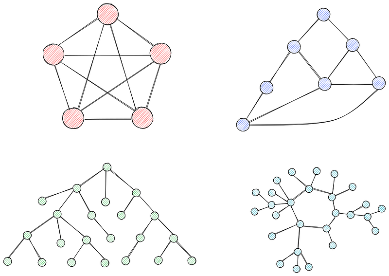
Graphs are collections of nodes (vertices) connected by edges. Nodes represent entities or points in a network, while edges represent the connection or relationships between them.
Graphs can be weighted or unweighted. In unweighted graphs, all edges have the same weight (often set to 1). In weighted graphs (you guessed it), each edge has a weight associated with it, often representing cost, distance, or time.
We will be using weighted graphs in the tutorial as they are required for Dijkstra’s algorithm.
A path in a graph refers to a sequence of nodes connected by edges, starting and ending at specific nodes. The shortest path, which we care about in this tutorial, is the path with the minimum total weight (distance, cost, etc.).
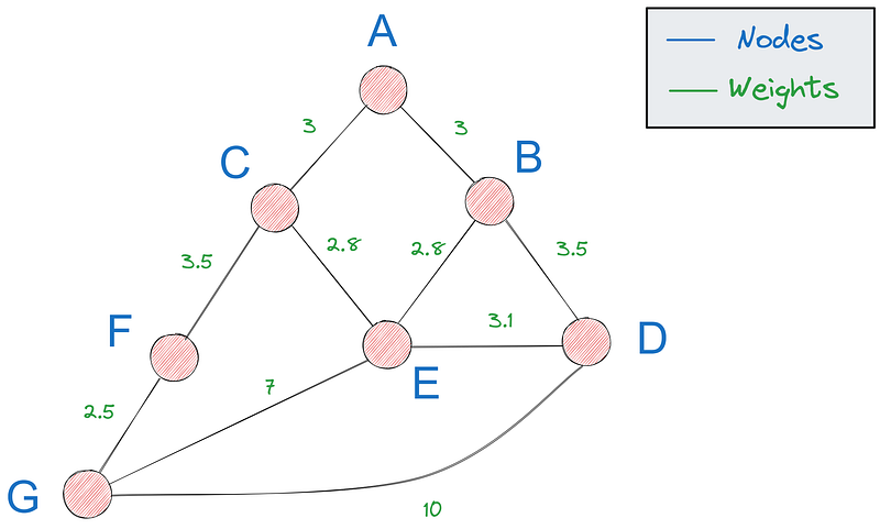
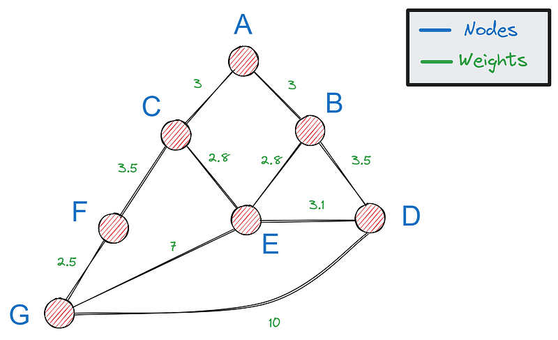
For the rest of the tutorial, we will be using the last graph we saw:

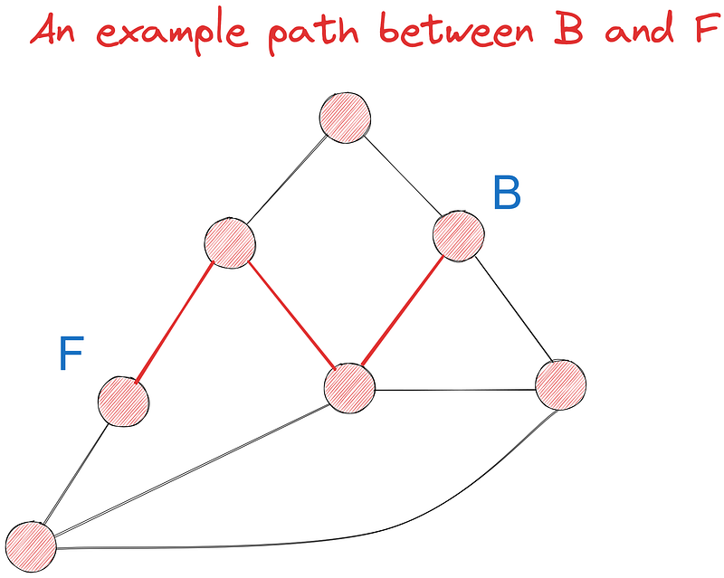
Let’s try to find the shortest path between points B and F using Dijkstra’s algorithm out of at least seven possible paths. Initially, we will do the task visually and implement it in code later.
First, we initialize the algorithm as follows:
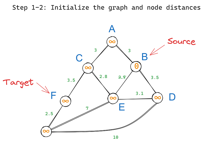
Then, we execute the following steps iteratively:
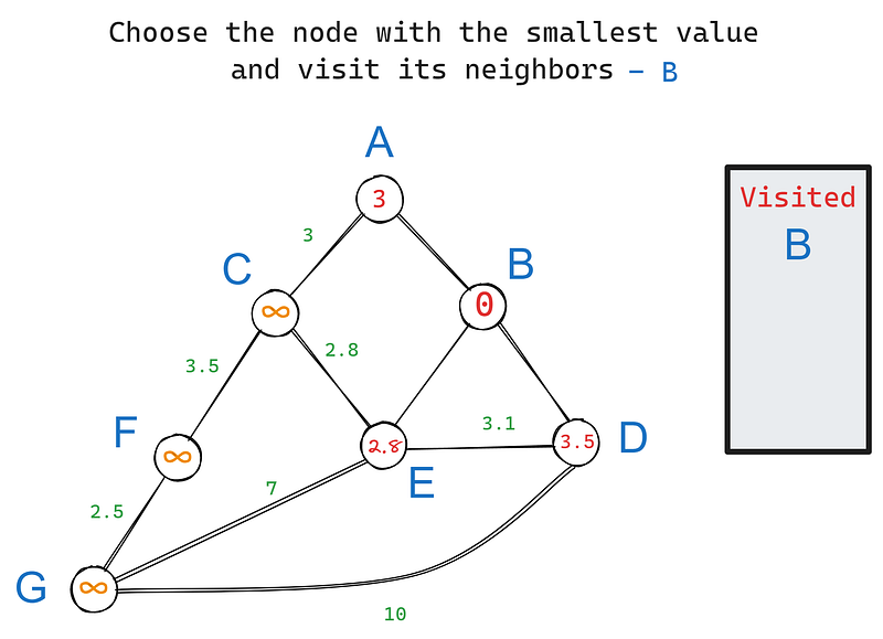
In our graph, B has three neighbors — A, D, and E. Let’s visit each one starting from the root node and update their values (iteration 1) based on their edge weights:
In iteration 2, we choose the node with the smallest value again, this time — E. Its neighbors are C, D, and G. B is excluded because we’ve already visited it. Let’s update the values of E’s neighbors:
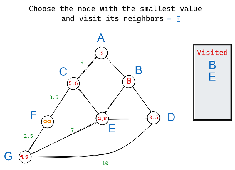
We set C’s value to 5.6 because its value is the cumulative sum of weights from B to C. The same goes for G. However, if you notice, D’s value remains 3.5 when it should have been 3.5 + 2.8 = 6.3, as with the other nodes.
The rule is that if the new cumulative sum is larger than the node’s current value, we won’t update it because the node already lists the shortest distance to the root. In this case, D’s current value of 3.5 already notes the shortest distance to B because they are neighbors.
We continue in this fashion until all nodes are visited. When that finally happens, we will have the shortest distance to each node from B and we can simply look up the value from B to F.
In summary, the steps are:
Now, to solidify your understanding of Dijkstra’s algorithm, we will learn to implement in Python step-by-step.
First, we need a way to represent graphs in Python— the most popular option is using a dictionary. If this is our graph:

We can represent it with the following dictionary:
graph = {
   "A": {"B": 3, "C": 3},
   "B": {"A": 3, "D": 3.5, "E": 2.8},
   "C": {"A": 3, "E": 2.8, "F": 3.5},
   "D": {"B": 3.5, "E": 3.1, "G": 10},
   "E": {"B": 2.8, "C": 2.8, "D": 3.1, "G": 7},
   "F": {"G": 2.5, "C": 3.5},
   "G": {"F": 2.5, "E": 7, "D": 10},
}
Each key of the dictionary is a node and each value is a dictionary containing the neighbors of the key and distances to it. Our graph has seven nodes which means the dictionary must have seven keys.
Other sources often refer to the above dictionary as a dictionary adjacency list. We will stick to that term from now on as well.
Graph classTo make our code more modular and easier to follow, we will implement a simple Graph class to represent graphs. Under the hood, it will use a dictionary adjacency list. It will also have a method to easily add connections between two nodes:
class Graph:
   def __init__(self, graph: dict = {}):
       self.graph = graph  # A dictionary for the adjacency list

   def add_edge(self, node1, node2, weight):
       if node1 not in self.graph:  # Check if the node is already added
           self.graph[node1] = {}  # If not, create the node
       self.graph[node1][node2] = weight  # Else, add a connection to its neighbor
Using this class, we can construct our graph iteratively from scratch like this:
G = Graph()

# Add A and its neighbors
G.add_edge("A", "B", 3)
G.add_edge("A", "C", 3)

# Add B and its neighbors
G.add_edge("B", "A", 3)
G.add_edge("B", "D", 3.5)
G.add_edge("B", "E", 2.8)

...
Or we can pass a dictionary adjacency list directly, which is a faster method:
# Use the dictionary we defined earlier
G = Graph(graph=graph)

G.graph
{'A': {'B': 3, 'C': 3},
'B': {'A': 3, 'D': 3.5, 'E': 2.8},
'C': {'A': 3, 'E': 2.8, 'F': 3.5},
'D': {'B': 3.5, 'E': 3.1, 'G': 10},
'E': {'B': 2.8, 'C': 2.8, 'D': 3.1, 'G': 7},
'F': {'G': 2.5, 'C': 3.5},
'G': {'F': 2.5, 'E': 7, 'D': 10}}
We create another class method — this time for the algorithm itself — shortest_distances:
class Graph:
   def __init__(self, graph: dict = {}):
       self.graph = graph

   # The add_edge method omitted for space

   def shortest_distances(self, source: str):
       # Initialize the values of all nodes with infinity
       distances = {node: float("inf") for node in self.graph}
       distances[source] = 0  # Set the source value to 0

       ...
The first thing we do inside the method is to define a dictionary that contains node-value pairs. This dictionary gets updated every time we visit a node and its neighbors. Like we mentioned in the visual explanation of the algorithm, the initial values of all nodes are set to infinity while the source’s value is 0.
When we finish writing the method, this dictionary will be returned, and it will have the shortest distances to all nodes from source. We will be able to find the distance from B to F like this:
# Sneak-peek - find the shortest paths from B
distances = G.shortest_distances("B")

to_F = distances["F"]
print(f"The shortest distance from B to F is {to_F}")
Now, we need a way to loop over the graph nodes based on the rules of Dijkstra's algorithm. If you remember, in each iteration, we need to choose the node with the smallest value and visit its neighbors.
You might say that we can simply loop over the dictionary keys:
for node in graph.keys():
   ...
This method doesn’t work as it doesn’t give us any way to sort nodes based on their value. So, simple arrays won’t suffice. To solve this portion of the problem, we will use something called a priority queue.
A priority queue is just like a regular list (array), but each of its elements has an extra value to represent their priority. This is a sample priority queue:
pq = [(3, "A"), (1, "C"), (7, "D")]This queue contains three elements — A, C, and D — and they each have a priority value that determines how operations are carried over the queue. Python provides a built-in heapq library to work with priority queues:
from heapq import heapify, heappop, heappushThe library has three functions we care about:
heapify: Turns a list of tuples with priority-value pairs into a priority queue.heappush: Adds an element to the queue with its associated priority.heappop: Removes and returns the element with the highest priority (the element with the smallest value).pq = [(3, "A"), (1, "C"), (7, "D")]
# Convert into a queue object
heapify(pq)
# Return the highest priority value
heappop(pq)
(1, 'C')As you can see, after we convert pq to a queue using heapify, we were able to extract C based on its priority. Let's try to push a value:
heappush(pq, (0, "B"))

heappop(pq)
(0, 'B')The queue is correctly updated based on the new element’s priority because heappop returned the new element with priority of 0.
Note that after we pop an item, it will no longer be part of the queue.
Now, getting back to our algorithm, after we initialize distances, we create a new priority queue that holds only the source node initially:
class Graph:
   def __init__(self, graph: dict = {}):
       self.graph = graph

   def shortest_distances(self, source: str):
       # Initialize the values of all nodes with infinity
       distances = {node: float("inf") for node in self.graph}
       distances[source] = 0  # Set the source value to 0

       # Initialize a priority queue
       pq = [(0, source)]
       heapify(pq)

       # Create a set to hold visited nodes
       visited = set()
The priority of each element inside pq will be its current value. We also initialize an empty set to record visited nodes.
while loopNow, we start iterating over all unvisited nodes using a while loop:
class Graph:
   def __init__(self, graph: dict = {}):
       self.graph = graph

   def shortest_distances(self, source: str):
       # Initialize the values of all nodes with infinity
       distances = {node: float("inf") for node in self.graph}
       distances[source] = 0  # Set the source value to 0

       # Initialize a priority queue
       pq = [(0, source)]
       heapify(pq)

       # Create a set to hold visited nodes
       visited = set()

       while pq:  # While the priority queue isn't empty
           current_distance, current_node = heappop(
               pq
           )  # Get the node with the min distance

           if current_node in visited:
               continue  # Skip already visited nodes
           visited.add(current_node)  # Else, add the node to visited set
While the priority queue isn’t empty, we keep popping the highest-priority node (with the minimum value) and extracting its value and name to current_distance and current_node. If the current_node is inside visited, we skip it. Otherwise, we mark it as visited and then, move on to visiting its neighbors:
while pq:  # While the priority queue isn't empty
   current_distance, current_node = heappop(pq)

   if current_node in visited:
       continue
   visited.add(current_node)

   for neighbor, weight in self.graph[current_node].items():
       # Calculate the distance from current_node to the neighbor
       tentative_distance = current_distance + weight
       if tentative_distance < distances[neighbor]:
           distances[neighbor] = tentative_distance
           heappush(pq, (tentative_distance, neighbor))

return distances
For each neighbor, we calculate the tentative distance from the current node by adding the neighbor’s current value to the connecting edge weight. Then, we check if the distance is smaller than the neighbor’s distance in distances. If yes, we update the distances dictionary and add the neighbor with its tentative distance to the priority queue.
That’s it! We have implemented Dijkstra's algorithm. Let’s test it:
G = Graph(graph)

distances = G.shortest_distances("B")
print(distances, "\n")

to_F = distances["F"]
print(f"The shortest distance from B to F is {to_F}")
{'A': 3, 'B': 0, 'C': 5.6, 'D': 3.5, 'E': 2.8, 'F': 9.1, 'G': 9.8}

The shortest distance from B to F is 9.1
So, the distance from B to F is 9.1. But wait: which path is it?
So, we only have the shortest distances not paths, which makes our graph look like this:
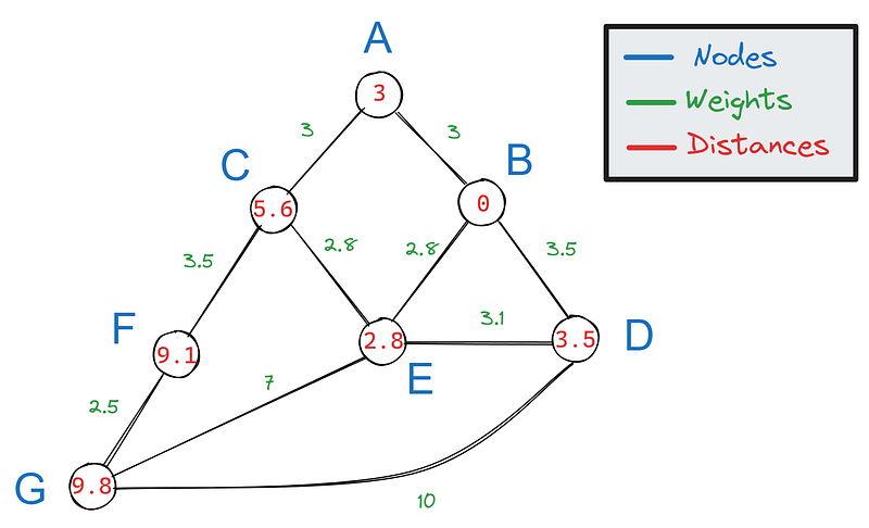
To construct the shortest path from the calculated shortest distance, we can backtrack our steps from the target. For each edge connected to F, we subtract its weight:
Then, we see if any of the results match the value of F’s neighbors. Only 5.6 matches C’s value, which means C is part of the shortest path.
We repeat this process again for C’s neighbors A and E:
Since 2.8 matches E’s value, it is part of the shortest path. E is also the neighbor of B, which make the shortest path between B and F — BECF.
Let’s add the implementation of this process to our class. The code itself is a bit different from the above explanation because it finds the shortest paths between B and all other nodes, not just F.
Also, it does this in reverse, but the idea is the same.
Add the following lines of code to the end of the shortest_distances method deleting the old return statement:
predecessors = {node: None for node in self.graph}

for node, distance in distances.items():
   for neighbor, weight in self.graph[node].items():
       if distances[neighbor] == distance + weight:
           predecessors[neighbor] = node

return distances, predecessors
When the code runs, the predecessors dictionary contains the immediate parent of each node involved in the shortest path to the source. Let's try it:
G = Graph(graph)

distances, predecessors = G.shortest_distances("B")

print(predecessors)
{'A': 'B', 'B': None, 'C': 'E', 'D': 'B', 'E': 'B', 'F': 'C', 'G': 'E'}First, let’s find the shortest path manually using the predecessors dictionary by backtracking from F:
# Check the predecessor of F
predecessors["F"]
'C' # It is C# Check the predecessor of C
predecessors["C"]
'E' # It is E# Check the predecessor of E
predecessors["E"]
'B' # It is BThere we go! The dictionary correctly tells us that the shortest path between B and F is BECF.
But we found the method semi-manually. We want a method that automatically returns the shortest path constructed from the predecessors dictionary from any source to any target. We define this method as shortest_path (add it to the end of the class):
def shortest_path(self, source: str, target: str):
   # Generate the predecessors dict
   _, predecessors = self.shortest_distances(source)

   path = []
   current_node = target

   # Backtrack from the target node using predecessors
   while current_node:
       path.append(current_node)
       current_node = predecessors[current_node]

   # Reverse the path and return it
   path.reverse()

   return path
By using the shortest_distances function, we generate the predecessors dictionary. Then, we start a while loop that goes back a node from the current node in each iteration until the source node is reached. Then, we return the list reversed, which contains the path from the source to the target.
Let’s test it:
G = Graph(graph)

G.shortest_path("B", "F")
['B', 'E', 'C', 'F']It works! Let’s try another one:
G.shortest_path("A", "G")['A', 'C', 'F', 'G']Right as rain.
In this tutorial, we learned one of the most fundamental algorithms in graph theory — Dijkstra’s. It is often the go-to algorithm for finding the shortest path between two points in graph-like structures. Due to its simplicity, it has applications in many industries such as:
I hope that implementing Dijkstra’s algorithm in Python sparked your interest in the wonderful world of graph algorithms. If you want to learn more, I highly recommend the following resources:
Continue Your Python Journey Today!
course
course
course
tutorial
Andrew Brooks
37 min
tutorial
Matthew Przybyla
12 min
tutorial
Amina Edmunds
7 min
tutorial
Abid Ali Awan
5 min
tutorial
Moez Ali
7 min