Introduction to Autoencoders: From The Basics to Advanced Applications in PyTorch

Traditional feedforward neural networks can be great at performing tasks such as classification and regression, but what if we would like to implement solutions such as signal denoising or anomaly detection? One way to do this is by using Autoencoders.

This tutorial provides a practical introduction to Autoencoders, including a hands-on example in PyTorch and some potential use cases.

You can follow along in the this DataLab workbook with all the code from the tutorial.

What are Autoencoders?

Autoencoders are a special type of unsupervised feedforward neural network (no labels needed!). The main application of Autoencoders is to accurately capture the key aspects of the provided data to provide a compressed version of the input data, generate realistic synthetic data, or flag anomalies.

Autoencoders are composed of 2 key fully connected feedforward neural networks (Figure 1):

• Encoder: compresses the input data to remove any form of noise and generates a latent space/bottleneck. Therefore, the output neural network dimensions are smaller than the input and can be adjusted as a hyperparameter in order to decide how much lossy our compression should be.
• Decoder: making use of only the compressed data representation from the latent space, tries to reconstruct with as much fidelity as possible the original input data (the architecture of this neural network is, therefore, generally a mirror image of the encoder). The “goodness” of the prediction can then be measured by calculating the reconstruction error between the input and output data using a loss function.

Repeating iteratively this process of passing data through the encoder and decoder and measuring the error to tune the parameters through backpropagation, the Autoencoder can, with time, correctly work with extremely difficult forms of data.

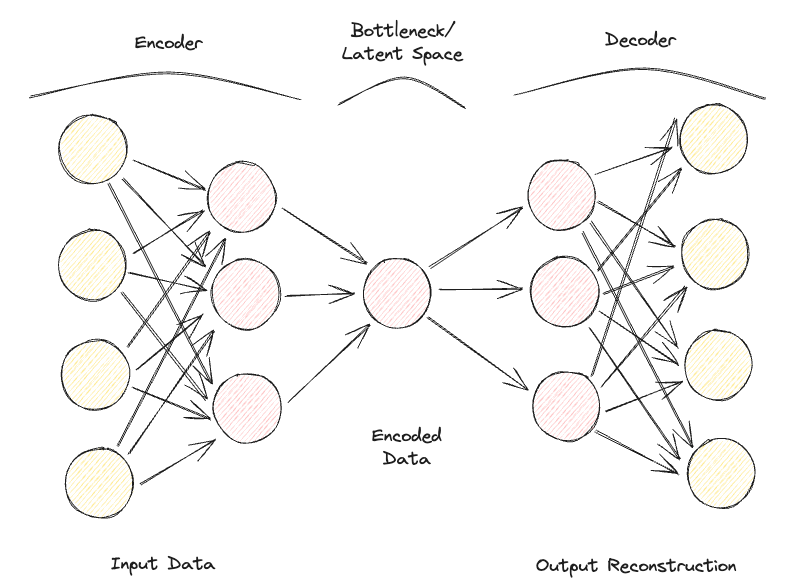
Figure 1: Autoencoder Architecture (Image by Author).

If an Autoencoder is provided with a set of input features completely independent of each other, then it would be really difficult for the model to find a good lower-dimensional representation without losing a great deal of information (lossy compression).

Autoencoders can, therefore, also be considered a dimensionality reduction technique, which compared to traditional techniques such as Principal Component Analysis (PCA), can make use of non-linear transformations to project data in a lower dimensional space. If you are interested in learning more about other Feature Extraction techniques, additional information is available in this feature extraction tutorial..

Additionally, compared to standard data compression algorithms like gzpi, Autoencoders can not be used as general-purpose compression algorithms but are handcrafted to work best just on similar data on which they have been trained on.

Some of the most common hyperparameters that can be tuned when optimizing your Autoencoder are:

• The number of layers for the Encoder and Decoder neural networks
• The number of nodes for each of these layers
• The loss function to use for the optimization process (e.g., binary cross-entropy or mean squared error)
• The size of the latent space (the smaller, the higher the compression, acting, therefore as a regularization mechanism)

Finally, Autoencoders can be designed to work with different types of data, such as tabular, time-series, or image data, and can, therefore, be designed to use a variety of layers, such as convolutional layers, for image analysis.

Ideally, a well-trained Autoencoder should be responsive enough to adapt to the input data in order to provide a tailor-made response but not so much as to just mimic the input data and not be able to generalize with unseen data (therefore overfitting).

Types of Autoencoders

Over the years, different types of Autoencoders have been developed:

• Undercomplete Autoencoder
• Sparse Autoencoder
• Contractive Autoencoder
• Denoising Autoencoder
• Convolutional Autoencoder
• Variational Autoencoder

Let’s explore each in more detail.

Undercomplete Autoencoder

This is the simplest version of an autoencoder. In this case, we don’t have an explicit regularization mechanism, but we ensure that the size of the bottleneck is always lower than the original input size to avoid overfitting. This type of configuration is typically used as a dimensionality reduction technique (more powerful than PCA since its also able to capture non-linearities in the data).

Sparse Autoencoder

A Sparse Autoencoder is quite similar to an Undercomplete Autoencoder, but their main difference lies in how regularization is applied. In fact, with Sparse Autoencoders, we don’t necessarily have to reduce the dimensions of the bottleneck, but we use a loss function that tries to penalize the model from using all its neurons in the different hidden layers (Figure 2).

This penalty is commonly referred to as a sparsity function, and it's quite different from traditional regularization techniques since it doesn’t focus on penalizing the size of the weights but the number of nodes activated.

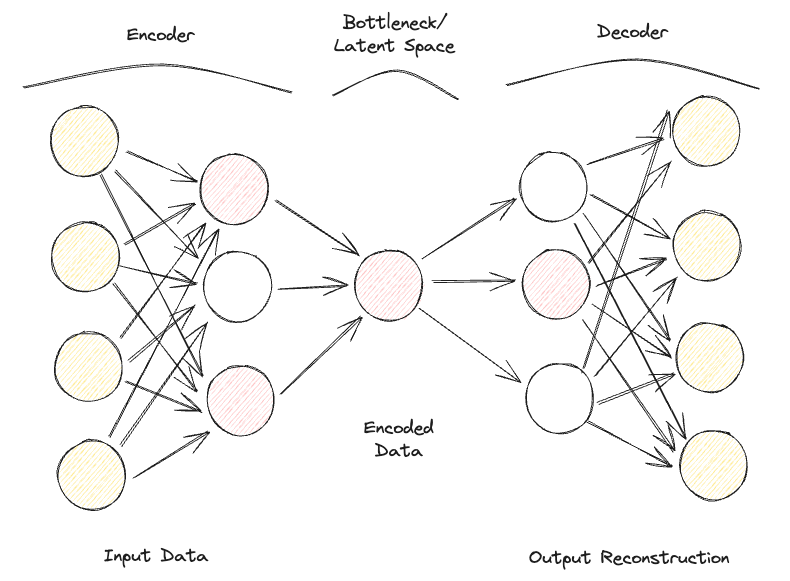
In this way, different nodes could specialize for different input types and be activated/deactivated depending on the specifics of the input data. This sparsity constraint can be induced by using L1 Regularization and KL divergence, effectively preventing the model from overfitting.

Contractive Autoencoder

The main idea behind Contractive Autoencoders is that given some similar inputs, their compressed representation should be quite similar (neighborhoods of inputs should be contracted in small neighborhood of outputs). In mathematical terms, this can be enforced by keeping input hidden layer activations derivatives small when fed similar inputs.

Denoising Autoencoder

With Denoising Autoencoders, the input and output of the model are no longer the same. For example, the model could be fed some low-resolution corrupted images and work for the output to improve the quality of the images. In order to assess the performance of the model and improve it over time, we would then need to have some form of labeled clean image to compare with the model prediction.

Convolutional Autoencoder

To work with image data, Convolutional Autoencoders replace traditional feedforward neural networks with Convolutional Neural Networks for both the encoder and decoder steps. Updating type of loss function, etc., this type of Autoencoder can also be made, for example, Sparse or Denoising, depending on your use case requirements.

Variational Autoencoder

In every type of Autoencoder considered so far, the encoder outputs a single value for each dimension involved. With Variational Autoencoders (VAE), we make this process instead probabilistic, creating a probability distribution for each dimension. The decoder can then sample a value from each distribution describing the different dimensions and construct the input vector, which it can then be used to reconstruct the original input data.

One of the main applications of Variational Autoencoders is for generative tasks. In fact, sampling the latent model from distributions can enable the decoder to create new forms of outputs that were previously not possible using a deterministic approach.

If you are interested in testing an online a Variational Autoencoder trained on the MNIST dataset, you can find a live example.

Autoencoder Hands-On Example

We are now ready to go through a practical demonstration of how Autoencoders can be used for dimensionality reduction. Our Deep Learning framework of choice for this exercise is going to be PyTorch.

The Kaggle Rain in Australia dataset is going to be used for this demonstration. All the code of this article is available in this DataLab workbook.

First of all, we import all the necessary libraries and remove any missing values and non-numeric columns (Figure 3).

import numpy as np
import pandas as pd
import torch
import torch.nn as nn
import torch.optim as optim
import matplotlib.pyplot as plt
from sklearn.preprocessing import StandardScaler, LabelEncoder
from mpl_toolkits.mplot3d import Axes3D

df = pd.read_csv("../input/weather-dataset-rattle-package/weatherAUS.csv")
df = df.drop(['Date', 'Location', 'WindDir9am',
             'WindGustDir', 'WindDir3pm'], axis=1)
df = df.dropna(how = 'any')
df.loc[df['RainToday'] == 'No', 'RainToday'] = 0
df.loc[df['RainToday'] == 'Yes', 'RainToday'] = 1
df.head()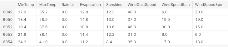

Figure 3: Sample of Dataset Columns (Image by Author).

At this point, we are ready to divide the data into features and labels, normalize the features, and convert the labels into a numeric format.

In this case, we have a starting feature set composed of 17 columns. The overall objective of the analysis would then be to correctly predict if it's going to rain the next day or not.

X, Y = df.drop('RainTomorrow', axis=1, inplace=False), df[['RainTomorrow']]
# Normalizing Data
scaler = StandardScaler()
X_scaled = scaler.fit_transform(X)

# Converting to PyTorch tensor
X_tensor = torch.FloatTensor(X_scaled)

# Converting string labels to numerical labels
label_encoder = LabelEncoder()
Y_numerical = label_encoder.fit_transform(Y.values.ravel())

In PyTorch, we can now define the Autoencoder model as a class and specify the encoder and decoder models with two linear layers.

# Defining Autoencoder model
class Autoencoder(nn.Module):
   def __init__(self, input_size, encoding_dim):
       super(Autoencoder, self).__init__()
       self.encoder = nn.Sequential(
           nn.Linear(input_size, 16),
           nn.ReLU(),
           nn.Linear(16, encoding_dim),
           nn.ReLU()
       )
       self.decoder = nn.Sequential(
           nn.Linear(encoding_dim, 16),
           nn.ReLU(),
           nn.Linear(16, input_size),
           nn.Sigmoid()
       )

   def forward(self, x):
       x = self.encoder(x)
       x = self.decoder(x)
       return x

Now that the model is set up, we can proceed to specify our encoding dimensions to be equal to 3 (to make it easy to plot them later on) and run through the training process.

# Setting random seed for reproducibility
torch.manual_seed(42)

input_size = X.shape[1]  # Number of input features
encoding_dim = 3  # Desired number of output dimensions
model = Autoencoder(input_size, encoding_dim)

# Loss function and optimizer
criterion = nn.MSELoss()
optimizer = optim.Adam(model.parameters(), lr=0.003)

# Training the autoencoder
num_epochs = 20
for epoch in range(num_epochs):
   # Forward pass
   outputs = model(X_tensor)
   loss = criterion(outputs, X_tensor)

   # Backward pass and optimization
   optimizer.zero_grad()
   loss.backward()
   optimizer.step()

   # Loss for each epoch
   print(f'Epoch [{epoch + 1}/{num_epochs}], Loss: {loss.item():.4f}')

# Encoding the data using the trained autoencoder
encoded_data = model.encoder(X_tensor).detach().numpy()

Epoch [1/20], Loss: 1.2443
Epoch [2/20], Loss: 1.2410
Epoch [3/20], Loss: 1.2376
Epoch [4/20], Loss: 1.2342
Epoch [5/20], Loss: 1.2307
Epoch [6/20], Loss: 1.2271
Epoch [7/20], Loss: 1.2234
Epoch [8/20], Loss: 1.2196
Epoch [9/20], Loss: 1.2156
Epoch [10/20], Loss: 1.2114
Epoch [11/20], Loss: 1.2070
Epoch [12/20], Loss: 1.2023
Epoch [13/20], Loss: 1.1974
Epoch [14/20], Loss: 1.1923
Epoch [15/20], Loss: 1.1868
Epoch [16/20], Loss: 1.1811
Epoch [17/20], Loss: 1.1751
Epoch [18/20], Loss: 1.1688
Epoch [19/20], Loss: 1.1622
Epoch [20/20], Loss: 1.1554

Finally, we can now plot the resulting embedding dimensions (Figure 4). As it can be seen in the image below, we successfully managed to reduce the dimensionality of our feature set from 17 dimensions to just 3, while still being able, to a good extent, to correctly separate in our 3-dimensional space samples between the different classes.

# Plotting the encoded data in 3D space
fig = plt.figure(figsize=(8, 8))
ax = fig.add_subplot(111, projection='3d')
scatter = ax.scatter(encoded_data[:, 0], encoded_data[:, 1],
                    encoded_data[:, 2], c=Y_numerical, cmap='viridis')

# Mapping numerical labels back to original string labels for the legend
labels = label_encoder.inverse_transform(np.unique(Y_numerical))
legend_labels = {num: label for num, label in zip(np.unique(Y_numerical),
                                                 labels)}

# Creating a custom legend with original string labels
handles = [plt.Line2D([0], [0], marker='o', color='w',
                    markerfacecolor=scatter.to_rgba(num),
                    markersize=10,
                    label=legend_labels[num]) for num in np.unique(Y_numerical)]
ax.legend(handles=handles, title="Raining Tomorrow?")

# Adjusting the layout to provide more space for labels
ax.xaxis.labelpad = 20
ax.yaxis.labelpad = 20

ax.set_xticks([])
ax.set_yticks([])
ax.set_zticks([])

# Manually adding z-axis label for better visibility
ax.text2D(0.05, 0.95, 'Encoded Dimension 3', transform=ax.transAxes,
         fontsize=12, color='black')

ax.set_xlabel('Encoded Dimension 1')
ax.set_ylabel('Encoded Dimension 2')
ax.set_title('Autoencoder Dimensionality Reduction')

plt.tight_layout()

plt.savefig('Rain_Prediction_Autoencoder.png')

plt.show()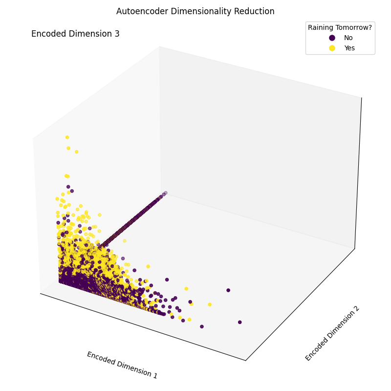

Figure 4: Resulting Encoded Dimensions (Image by Author).

Real-life Applications of Autoencoders

Image Compression/Denoising

One of the main applications of Autoencoders is to compress images to reduce their overall file size while trying to keep as much of the valuable information as possible or restore images that have been degraded over time.

Anomaly Detection

Since Autoencoders are good at distinguishing essential characteristics of data from noise, they can be used in order to detect anomalies (e.g., if an image has been photoshopped, if there are unusual activities in a network, etc.)

Data Generation

Variational Autoencoders and Generative Adversarial Networks (GAN) are frequently used in order to generate synthetic data (e.g., realistic images of people).

Conclusion

In conclusion, Autoencoders can be a really flexible tool to power different forms of use cases. In particular, Variational Autoencoders and the creation of GANs opened the door to the development of Generative AI, offering us the first glimpses of how AI can be used to generate new forms of content never seen before.

This tutorial was an introduction to the field of Autoencoders, although there is still a lot to learn! DataCamp has a wide variety of resources about this topic, such as how to implement Autoencoders in Keras or use them as a classifier!