NLP with PyTorch: A Comprehensive Guide

Introduction to NLP and PyTorch

Natural Language Processing (NLP) is a critical component of modern AI, enabling machines to understand and respond to human language. As digital interactions proliferate, NLP's importance grows. PyTorch, a popular open-source machine learning library, provides robust tools for NLP tasks due to its flexibility and efficient tensor computations. Its dynamic computational graph also aids in easily modifying and building complex models, making it ideal for our tutorial.

If you are interested in learning more about NLP, Check out our Natural Language Processing in Python skill track, or if you prefer to learn the art of NLP in R instead, check out the Introduction to Natural Language Processing in R course on DataCamp.

Setting up the Environment

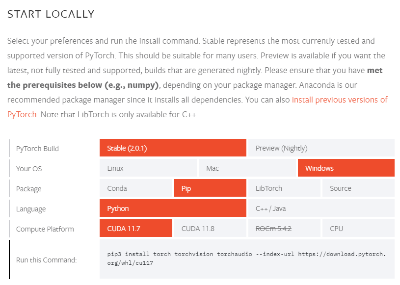
Setting up the PyTorch environment can be challenging at times due to factors such as operating system, package manager preference, programming language, and computing platform. The installation process may vary slightly depending on these factors, requiring you to run specific commands.

To obtain the appropriate install command, you can visit PyTorch's official get started page, where you can select your preferences and receive the necessary instructions.

We will use DataCamp Workspaces for this tutorial. The complete code for the training sentiment analysis model using PyTorch is available here if you want to follow along.

Introduction to Tensors

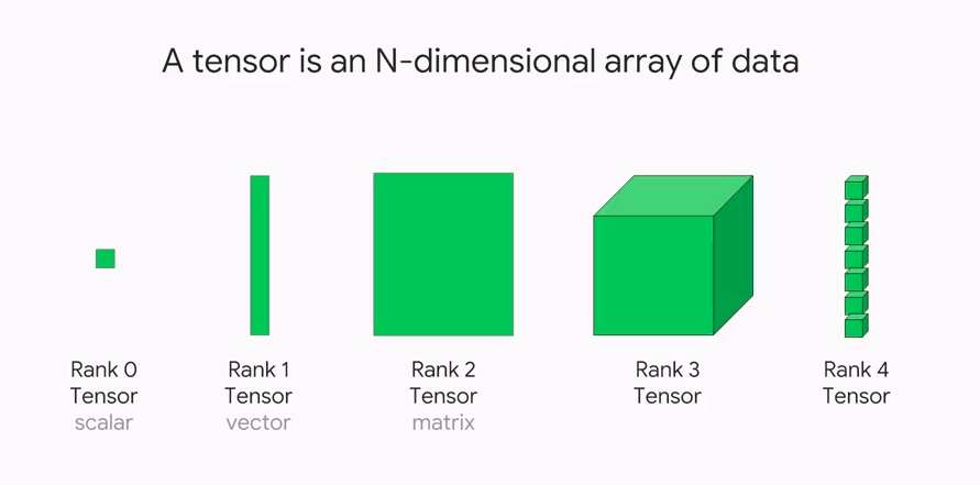
Tensors are fundamental data structures in mathematics and physics that generalize scalars, vectors, and matrices. They are multi-dimensional arrays capable of storing and manipulating large amounts of numerical data efficiently. Tensors have a defined shape, size, and data type, making them versatile for various computational operations.

In the context of PyTorch, tensors are the primary building blocks and data representation objects. Tensors in PyTorch are similar to NumPy arrays but come with additional functionalities and optimizations specifically designed for deep learning computations. PyTorch's tensor operations leverage hardware acceleration, such as GPUs, for efficient computation of complex neural networks.

Tensors play a critical role in natural language processing (NLP) tasks due to the inherent sequential and hierarchical nature of language data.

NLP involves processing and understanding textual information. Tensors enable the representation and manipulation of text data by encoding words, sentences, or documents as numerical vectors.

This numerical representation allows deep learning models to process and learn from textual data effectively. Tensors enable the efficient handling of large-scale language datasets, facilitate the training of neural networks, and enable advanced techniques like attention mechanisms for more accurate NLP models.

Word Embeddings

Word embeddings are dense vector representations of words in a continuous vector space. They aim to capture semantic and syntactic relationships between words, allowing for better understanding and contextualization of textual data. By representing words as numerical vectors, word embeddings capture semantic similarities and differences, enabling algorithms to work with words as meaningful numerical inputs.

In simple terms, embeddings are a clever way of representing words as numbers. These numbers have special meanings that capture how words are related to each other. It's like a secret code that helps computers understand and work with words more easily.

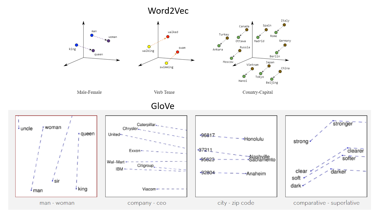
Word2Vec and GloVe are two popular methods for generating word embeddings. Word2Vec is a neural network-based model that learns word representations by predicting the surrounding words given a target word (continuous bag of words - CBOW) or predicting the target word based on its context (skip-gram).

GloVe (Global Vectors for Word Representation) is a count-based method that constructs word vectors based on the co-occurrence statistics of words in a large corpus. It captures global word relationships and often leads to better performance in word analogy tasks.

NLP Model Architecture

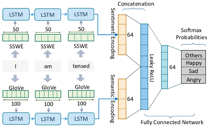
Example Model Architecture for Sentiment Analysis Task.

Sentiment Analysis is a common task in NLP where the objective is to understand the sentiment expressed in a piece of text, often classified as positive, negative, or neutral. To tackle this task, a simple recurrent neural network (RNN) or a more advanced version called long short-term memory (LSTM) can be used.

RNNs

RNN architecture processes the text sequentially, where each word is input one after another. The network maintains a hidden state that changes with each word input, capturing the information from the sequence processed so far.

This hidden state acts as the memory of the network. However, standard RNNs struggle with long sequences due to what's known as the vanishing gradient problem, where the contribution of information decays geometrically over time, making the network forget the earlier inputs. You can learn more about recurrent neural networks in our RNN tutorial. 

LSTMs

To combat this, LSTM, a variant of RNN, was developed. An LSTM maintains a longer context or 'memory' by having a more complex internal structure in its hidden state. It has a series of 'gates' (input, forget, and output gate) that control the flow of information in and out of the memory state.

The input gate determines how much of the incoming information should be stored in the memory state. The forget gate decides what information should be discarded, and the output gate defines how much of the internal state is exposed to the next LSTM unit in the sequence.

RNN or LSTM model would take a sequence of words in a sentence or document as the input. Each word is typically represented as a dense vector, or embedding, which captures the semantic meaning of the word.

The network processes the sequence word by word, updating its internal state based on the current word and the previous state.

The final state of the network is then used to predict the sentiment. It is passed through a fully connected layer, followed by a softmax activation function to output a probability distribution over the sentiment classes (e.g., positive, negative, neutral).

The class with the highest probability is chosen as the model's prediction.

This is a basic setup and can be further enhanced with techniques such as bidirectional LSTMs (which process the sequence in both directions), and attention mechanisms (which allow the model to focus on important parts of the sequence), among others.

Training LSTM Model in PyTorch for Sentiment Analysis

End-to-End Python Code example to build Sentiment Analysis Model using PyTorch

1. Load the dataset

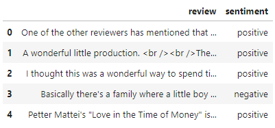
In this example, we will be using the IMDB dataset of 50K Movie reviews. The goal is to train a LSTM model to predict the sentiment. There are two possible values: 'positive’ and ‘negative’. Hence this is a binary classification task.

file_name = 'IMDB Dataset.csv'
df = pd.read_csv(file_name)
df.head()

2. Exploratory data analysis

X,y = df['review'].values,df['sentiment'].values
x_train,x_test,y_train,y_test = train_test_split(X,y,stratify=y)
print(f'train data shape: {x_train.shape}')
print(f'test data shape: {x_test.shape}')


dd = pd.Series(y_train).value_counts()
sns.barplot(x=np.array(['negative','positive']),y=dd.values)
plt.show()

Output:

>>> train data shape: (37500,)

>>> test data shape: (12500,)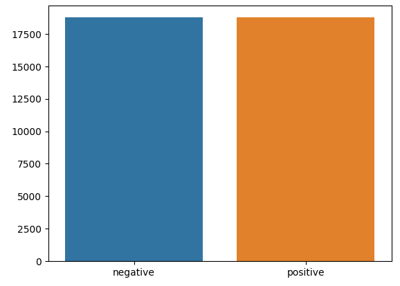

3. Text preprocessing

Text preprocessing and tokenization is a critical first step. First, we clean up the text data by removing punctuation, extra spaces, and numbers.

We then transform sentences into individual words, remove common words (known as "stop words"), and keep track of the 1000 most frequently used words in the dataset. These words are then assigned a unique identifier, forming a dictionary for one-hot encoding.

The code essentially is converting the original text sentences into sequences of these unique identifiers, translating human language into a format that a machine learning model can understand.

def preprocess_string(s):
    # Remove all non-word characters (everything except numbers and letters)
    s = re.sub(r"[^\w\s]", '', s)
    # Replace all runs of whitespaces with no space
    s = re.sub(r"\s+", '', s)
    # replace digits with no space
    s = re.sub(r"\d", '', s)
    return s


def tokenize(x_train,y_train,x_val,y_val):
    word_list = []


    stop_words = set(stopwords.words('english'))
    for sent in x_train:
        for word in sent.lower().split():
            word = preprocess_string(word)
            if word not in stop_words and word != '':
                word_list.append(word)
 
    corpus = Counter(word_list)
    # sorting on the basis of most common words
    corpus_ = sorted(corpus,key=corpus.get,reverse=True)[:1000]
    # creating a dict
    onehot_dict = {w:i+1 for i,w in enumerate(corpus_)}
   
    # tokenize
    final_list_train,final_list_test = [],[]
    for sent in x_train:
            final_list_train.append([onehot_dict[preprocess_string(word)] for word in sent.lower().split()
                                     if preprocess_string(word) in onehot_dict.keys()])
    for sent in x_val:
            final_list_test.append([onehot_dict[preprocess_string(word)] for word in sent.lower().split()
                                    if preprocess_string(word) in onehot_dict.keys()])
           
    encoded_train = [1 if label =='positive' else 0 for label in y_train]  
    encoded_test = [1 if label =='positive' else 0 for label in y_val]
    return np.array(final_list_train), np.array(encoded_train),np.array(final_list_test), np.array(encoded_test),onehot_dict


x_train,y_train,x_test,y_test,vocab = tokenize(x_train,y_train,x_test,y_test)

Let’s analyze the token length in x_train.

rev_len = [len(i) for i in x_train]
pd.Series(rev_len).hist()

4. Preparing the data for the model

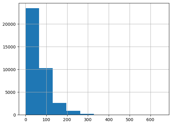
Given the variable token lengths of each review, it's necessary to standardize them for consistency. As the majority of reviews contain less than 500 tokens, we'll establish 500 as the fixed length for all reviews.

def padding_(sentences, seq_len):
    features = np.zeros((len(sentences), seq_len),dtype=int)
    for ii, review in enumerate(sentences):
        if len(review) != 0:
            features[ii, -len(review):] = np.array(review)[:seq_len]
    return features


x_train_pad = padding_(x_train,500)
x_test_pad = padding_(x_test,500)

Next, we use DataLoader class to create the final dataset for model training.

# create Tensor datasets
train_data = TensorDataset(torch.from_numpy(x_train_pad), torch.from_numpy(y_train))
valid_data = TensorDataset(torch.from_numpy(x_test_pad), torch.from_numpy(y_test))


# dataloaders
batch_size = 50


# make sure to SHUFFLE your data
train_loader = DataLoader(train_data, shuffle=True, batch_size=batch_size)
valid_loader = DataLoader(valid_data, shuffle=True, batch_size=batch_size)


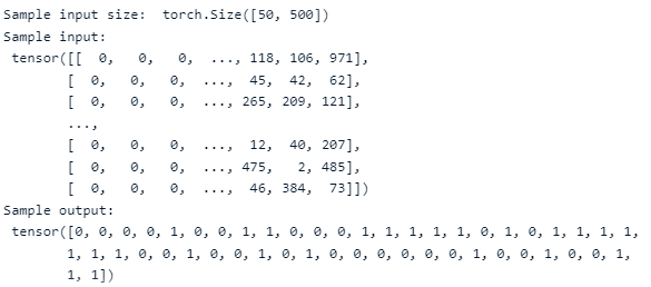
# obtain one batch of training data
dataiter = iter(train_loader)
sample_x, sample_y = next(dataiter)


print('Sample input size: ', sample_x.size()) # batch_size, seq_length
print('Sample input: \n', sample_x)
print('Sample output: \n', sample_y)

Output:

5. Define the LSTM model

This part of the code defines a sentiment analysis model using a recurrent neural network (RNN) architecture, specifically a type of RNN called Long Short-Term Memory (LSTM) as we mentioned above. The SentimentRNN class is a PyTorch model that starts with an embedding layer, which transforms word indices into a dense representation that captures the semantic meaning of words. This is followed by an LSTM layer that processes the sequence of word embeddings.

The LSTM's hidden state is passed through a dropout layer (for regularizing the model and preventing overfitting) and a fully connected layer, which maps the LSTM outputs to the final prediction. The prediction is then passed through a sigmoid activation function, converting raw output values into probabilities. The forward method defines the forward pass of data through this network, and the init_hidden method initializes the hidden states of the LSTM layer to zeros.

class SentimentRNN(nn.Module):
    def __init__(self,no_layers,vocab_size,hidden_dim,embedding_dim,drop_prob=0.5):
        super(SentimentRNN,self).__init__()
 
        self.output_dim = output_dim
        self.hidden_dim = hidden_dim
 
        self.no_layers = no_layers
        self.vocab_size = vocab_size
   
        # embedding and LSTM layers
        self.embedding = nn.Embedding(vocab_size, embedding_dim)
       
        #lstm
        self.lstm = nn.LSTM(input_size=embedding_dim,hidden_size=self.hidden_dim,
                           num_layers=no_layers, batch_first=True)
       
        # dropout layer
        self.dropout = nn.Dropout(0.3)
   
        # linear and sigmoid layer
        self.fc = nn.Linear(self.hidden_dim, output_dim)
        self.sig = nn.Sigmoid()
       
    def forward(self,x,hidden):
        batch_size = x.size(0)
        # embeddings and lstm_out
        embeds = self.embedding(x)  # shape: B x S x Feature   since batch = True
        #print(embeds.shape)  #[50, 500, 1000]
        lstm_out, hidden = self.lstm(embeds, hidden)
       
        lstm_out = lstm_out.contiguous().view(-1, self.hidden_dim)
       
        # dropout and fully connected layer
        out = self.dropout(lstm_out)
        out = self.fc(out)
       
        # sigmoid function
        sig_out = self.sig(out)
       
        # reshape to be batch_size first
        sig_out = sig_out.view(batch_size, -1)


        sig_out = sig_out[:, -1] # get last batch of labels
       
        # return last sigmoid output and hidden state
        return sig_out, hidden
       
    def init_hidden(self, batch_size):
        ''' Initializes hidden state '''
        # Create two new tensors with sizes n_layers x batch_size x hidden_dim,
        # initialized to zero, for hidden state and cell state of LSTM
        h0 = torch.zeros((self.no_layers,batch_size,self.hidden_dim)).to(device)
        c0 = torch.zeros((self.no_layers,batch_size,self.hidden_dim)).to(device)
        hidden = (h0,c0)
        return hidden 

Now we will initialize the SentimentRNN class that we defined above with the required parameters.

no_layers = 2
vocab_size = len(vocab) + 1 #extra 1 for padding
embedding_dim = 64
output_dim = 1
hidden_dim = 256


model = SentimentRNN(no_layers,vocab_size,hidden_dim,embedding_dim,drop_prob=0.5)


#moving to gpu
model.to(device)
print(model)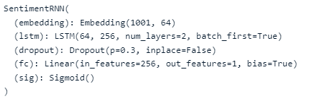

The final step before starting the training process is to define loss and optimization functions. This part focuses on defining the loss function, optimization method, and a utility function for accuracy calculation for our sentiment analysis model.

The loss function used is Binary Cross-Entropy Loss (nn.BCELoss), which is commonly used for binary classification tasks like this one. The optimization method is Adam (torch.optim.Adam), a popular choice due to its efficiency and low memory requirements. The learning rate for Adam is set to 0.001.

The acc function is a helper function designed to calculate the accuracy of our model's predictions. It rounds off the predicted probabilities to the nearest integer (0 or 1), compares these predictions to the actual labels, and then calculates the percentage of correct predictions.

# loss and optimization functions


lr=0.001


criterion = nn.BCELoss()


optimizer = torch.optim.Adam(model.parameters(), lr=lr)


# function to predict accuracy
def acc(pred,label):
    pred = torch.round(pred.squeeze())
    return torch.sum(pred == label.squeeze()).item()

6. Start training

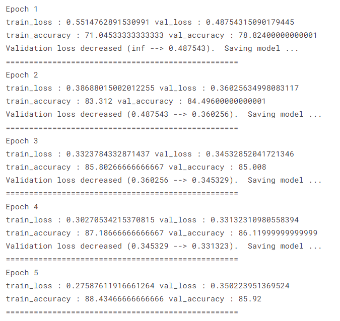
This is the part of the code where the sentiment analysis model is trained and validated. Each epoch (iteration) involves a training phase and a validation phase. During the training phase, the model learns by adjusting its parameters to minimize the loss.

In the validation phase, the model's performance is evaluated on a separate dataset to ensure it's learning generalized patterns and not just memorizing the training data.

The training loop starts by initializing the hidden states of the LSTM and setting the model to training mode. For each batch of data, the model's predictions are compared to the actual labels to compute the loss, which is then backpropagated to update the model's parameters.

Gradients are clipped to a maximum value to prevent them from getting too large, a common issue in training RNNs and LSTMs.

In the validation loop, the model is set to evaluation mode, and its performance is assessed using the validation data without updating any parameters. For both training and validation phases, the code tracks the loss and accuracy for each epoch.

If the validation loss improves, the current model's parameters are saved, capturing the best model found during training.

Finally, after each epoch, the average loss and accuracy for that epoch are printed out, giving insight into the model's learning progress.

clip = 5
epochs = 5
valid_loss_min = np.Inf
# train for some number of epochs
epoch_tr_loss,epoch_vl_loss = [],[]
epoch_tr_acc,epoch_vl_acc = [],[]


for epoch in range(epochs):
    train_losses = []
    train_acc = 0.0
    model.train()
    # initialize hidden state
    h = model.init_hidden(batch_size)
    for inputs, labels in train_loader:
       
        inputs, labels = inputs.to(device), labels.to(device)  
        # Creating new variables for the hidden state, otherwise
        # we'd backprop through the entire training history
        h = tuple([each.data for each in h])
       
        model.zero_grad()
        output,h = model(inputs,h)
       
        # calculate the loss and perform backprop
        loss = criterion(output.squeeze(), labels.float())
        loss.backward()
        train_losses.append(loss.item())
        # calculating accuracy
        accuracy = acc(output,labels)
        train_acc += accuracy
        #`clip_grad_norm` helps prevent the exploding gradient problem in RNNs / LSTMs.
        nn.utils.clip_grad_norm_(model.parameters(), clip)
        optimizer.step()
       
    val_h = model.init_hidden(batch_size)
    val_losses = []
    val_acc = 0.0
    model.eval()
    for inputs, labels in valid_loader:
            val_h = tuple([each.data for each in val_h])


            inputs, labels = inputs.to(device), labels.to(device)


            output, val_h = model(inputs, val_h)
            val_loss = criterion(output.squeeze(), labels.float())


            val_losses.append(val_loss.item())
           
            accuracy = acc(output,labels)
            val_acc += accuracy
           
    epoch_train_loss = np.mean(train_losses)
    epoch_val_loss = np.mean(val_losses)
    epoch_train_acc = train_acc/len(train_loader.dataset)
    epoch_val_acc = val_acc/len(valid_loader.dataset)
    epoch_tr_loss.append(epoch_train_loss)
    epoch_vl_loss.append(epoch_val_loss)
    epoch_tr_acc.append(epoch_train_acc)
    epoch_vl_acc.append(epoch_val_acc)
    print(f'Epoch {epoch+1}')
    print(f'train_loss : {epoch_train_loss} val_loss : {epoch_val_loss}')
    print(f'train_accuracy : {epoch_train_acc*100} val_accuracy : {epoch_val_acc*100}')
    if epoch_val_loss <= valid_loss_min:
        torch.save(model.state_dict(), 'state_dict.pt')
        print('Validation loss decreased ({:.6f} --> {:.6f}).  Saving model ...'.format(valid_loss_min,epoch_val_loss))
        valid_loss_min = epoch_val_loss
    print(25*'==')

Output:

7. Model evaluation

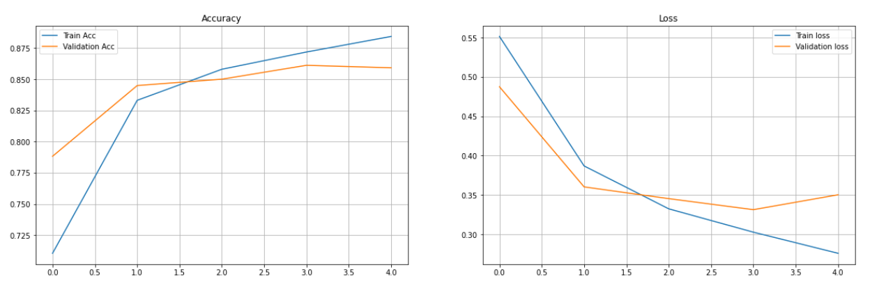
This part of the code is generating two plots to visually represent the training and validation accuracy and loss over the course of model training. The first subplot displays a line graph of the training and validation accuracy after each epoch. This plot is useful for observing how well the model is learning and generalizing over time.

The second subplot displays a line graph of the training and validation loss. This helps us see whether our model is overfitting, underfitting, or fitting just right.

fig = plt.figure(figsize = (20, 6))
plt.subplot(1, 2, 1)
plt.plot(epoch_tr_acc, label='Train Acc')
plt.plot(epoch_vl_acc, label='Validation Acc')
plt.title("Accuracy")
plt.legend()
plt.grid()
   
plt.subplot(1, 2, 2)
plt.plot(epoch_tr_loss, label='Train loss')
plt.plot(epoch_vl_loss, label='Validation loss')
plt.title("Loss")
plt.legend()
plt.grid()


plt.show()

Output:

8. Inference / Prediction

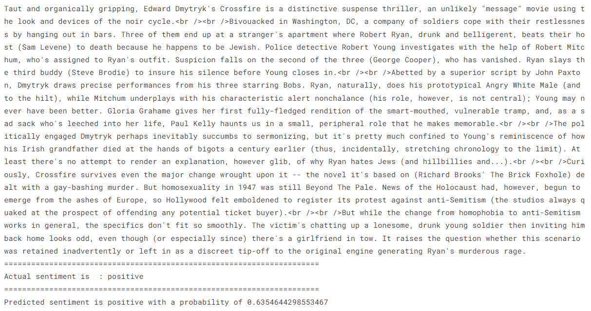
In this part, we create a function predict_text for predicting the sentiment of a given text, and a demonstration of its use. The predict_text function takes as input a string of text, transforms it into a sequence of word indices (according to a pre-defined vocabulary), and prepares it for input into the model by padding and reshaping. The function then initializes the hidden states of the LSTM, feeds the input into the model, and returns the model's output probability of the raw text.

def predict_text(text):
        word_seq = np.array([vocab[preprocess_string(word)] for word in text.split()
                         if preprocess_string(word) in vocab.keys()])
        word_seq = np.expand_dims(word_seq,axis=0)
        pad =  torch.from_numpy(padding_(word_seq,500))
        inputs = pad.to(device)
        batch_size = 1
        h = model.init_hidden(batch_size)
        h = tuple([each.data for each in h])
        output, h = model(inputs, h)
        return(output.item())


index = 30
print(df['review'][index])
print('='*70)
print(f'Actual sentiment is  : {df["sentiment"][index]}')
print('='*70)
pro = predict_text(df['review'][index])
status = "positive" if pro > 0.5 else "negative"
pro = (1 - pro) if status == "negative" else pro
print(f'Predicted sentiment is {status} with a probability of {pro}')

Output:

This entire notebook was developed using DataCamp Workspaces and can be accessed at this Workspace. It's important to remember that executing the code could take a substantial amount of time if you're using a CPU. However, the utilization of a GPU could significantly decrease the training time.

Next Steps / Improving the Model

Improving an NLP model often involves multiple strategies tailored to the specific requirements and constraints of the task at hand. Hyperparameter tuning is a common approach that involves adjusting parameters such as learning rate, batch size, or the number of layers in a neural network.

These hyperparameters can significantly influence the model's performance and are typically optimized through techniques like grid search or random search.

Transfer learning, particularly with models like BERT or GPT, has shown significant potential in improving NLP tasks. These models are pre-trained on large corpora of text and then fine-tuned on a specific task, allowing them to leverage the general language understanding they've gained during pre-training. This approach has consistently led to state-of-the-art results in a wide range of NLP tasks, including sentiment analysis.

Real-World Applications of NLP with PyTorch

The use of Natural Language Processing (NLP) models, particularly those implemented using frameworks like PyTorch, has seen widespread adoption in real-world applications, revolutionizing various aspects of our digital lives.

Chatbots have become an integral part of customer service platforms, leveraging NLP models to understand and respond to user queries. These models can process natural language input, infer the intent, and generate human-like responses, providing seamless interaction experiences.

In the realm of recommendation systems, NLP models help analyze user reviews and comments to understand user preferences, thereby enhancing the personalization of recommendations.

Sentiment analysis tools also rely heavily on NLP. These tools can scrutinize social media posts, customer reviews, or any text data and infer the sentiment behind them. Businesses often use these insights for market research or to gauge public sentiment about their products or services, allowing them to make data-driven decisions.

Discover more real-world use cases for using Google BERT in this Natural Language Processing Tutorial.

Conclusion

PyTorch offers a powerful and flexible platform for building NLP models. In this tutorial, we have walked through the process of developing a sentiment analysis model using an LSTM architecture, highlighting key steps such as preprocessing text data, building the model, training and validating it, and finally making predictions on unseen data.

This is just the tip of the iceberg for what is possible with NLP and PyTorch. NLP has vast applications, from chatbots and recommendation systems to sentiment analysis tools and beyond.

The continuous evolution in the field, especially with the advent of transfer learning models such as BERT and GPT, opens up even more exciting possibilities for future exploration. Mastering NLP with PyTorch is challenging yet rewarding, as it opens up a new dimension of understanding and interacting with the world around us.

If you are interested in deep diving into PyTorch, check out our Deep Learning with PyTorch course. Here, you’ll start with an introduction to PyTorch, exploring the PyTorch library and its applications for neural networks and deep learning. Next, you’ll cover artificial neural networks and learn how to train them using real data.