Precision-Recall Curve in Python Tutorial

Machine learning (ML) algorithms are increasingly used to automate mundane tasks and identify hidden patterns in data. But they are inherently probabilistic, meaning their predictions aren’t always correct. Hence, you need a way to estimate the validity of your ML model to establish trust in such systems. 

Evaluation metrics such as accuracy, precision, recall, mean squared error (MSE), mean absolute percentage error (MAPE), and similar are commonly used to measure the model performance. Different metrics help you measure performance through different criteria and lenses. 

These metrics also ensure that the model is constantly improving on learning its intended task. After all, if you can’t measure, you can’t improve the performance of the ML system.

Accuracy is one such metric that is easy to understand and works well with a balanced dataset, i.e., the one where all classes have equal representation. However, the real-world phenomena are not equally distributed; hence such balanced datasets are hard to find. Accuracy primarily concerns around finding whether the majority of the instances are correctly identified, irrespective of the class they belong to. For important rare events like a fraudulent transaction or a click on an ad impression, accuracy misrepresents a model just predicting everything as the negative class i.e. no fraud or no clicks. Owing to such limitations, accuracy is not the most appropriate metric. So, which metric should we use instead to measure the performance of our models?

Precision and recall are widely used metrics to evaluate the performance of an imbalanced classification model, such as predicting customer churn. 

Precision and Recall, Explained

Precision refers to the confidence with which a positive class is predicted as positive, while recall measures how well the model identifies the number of positive class instances from the dataset. Note that the positive class is the class of interest.

Empirically speaking, precision and recall are best understood with the help of a confusion matrix which consists of four key terms:

• True Positive (TP): Number of correctly identified positive class instances
• False Positive (FP): Number of negative class instances wrongly identified as positive class instances
• True Negative (TN): Number of correctly identified negative class instances
• False Negative (FN): Number of positive class instances wrongly identified as negative class instances

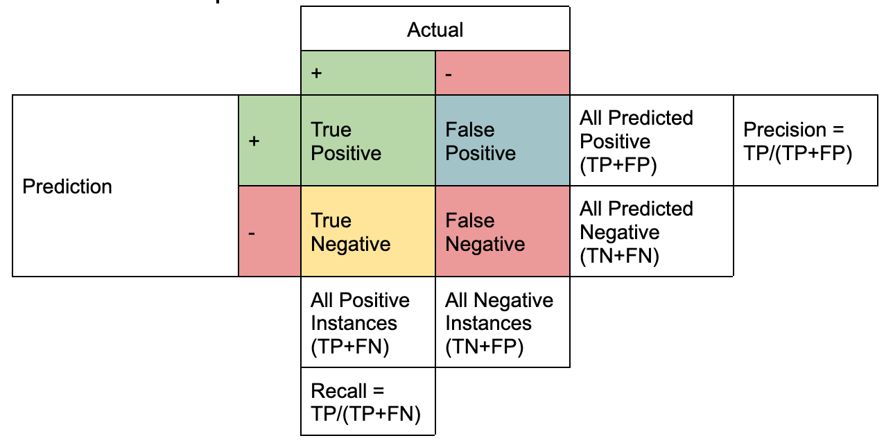
Representation created by the Author

Precision and Recall are a mathematical expression of these four terms where:

Precision is the proportion of TP to all the instances of positive predictions (TP+FP). Recall is the proportion of TP from all the positive instances (TP+FN).

It is further simplified using the following notation highlighting the difference between the two. Essentially, both the metrics have the same numerator, which is the intersection of actual positive instances with that of positively predicted instances, i.e., TP.

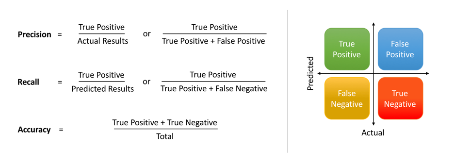
Image by Shruti Saxena

The differentiator is in the denominator where Precision considers all positively predicted instances (TP+FP), as against actual positive instances (TP+FN) in the case of Recall. 

Intuition Behind Precision and Recall 

There is a reason the confusion matrix is named so – it is indeed confusing when you try to grasp these concepts for the first time. 

So, let us internalize the concept with the help of an example. Let’s say you own a steel plant where the factory extracts iron from the iron ore and mixes it with other minerals and elements (sometimes unintentionally). Focusing on the extraction part, you have a few choices regarding the purity of metal extracted and waste produced during the process as given below:

Scenario 1: You want to just prioritize the purity of the extracted iron, irrespective of how much metal is wasted in the process.

Scenario 2: You want to maximize the efficiency, that is, the amount of iron extracted per unit of ore, disregarding the purity of the extracted metal.

Scenario 3: You want the best of both worlds, that is, by keeping the extracted metal purity as high as possible while reducing waste (maximizing the iron extracted per unit of ore).

Think of the blast furnace or electric arc furnace as the modeling options that provide different results (purity of iron ore and wastage). Let’s say one of the methods of extraction provides 97.5% pure iron and loses 4% of the iron in the sludge. Thus we can define our precision as the fraction of pure iron in the extracted metal, i.e., 97.5%, while recall is the amount of iron extracted from all the iron available in the ore, which is 96% (4% of all iron is wasted).

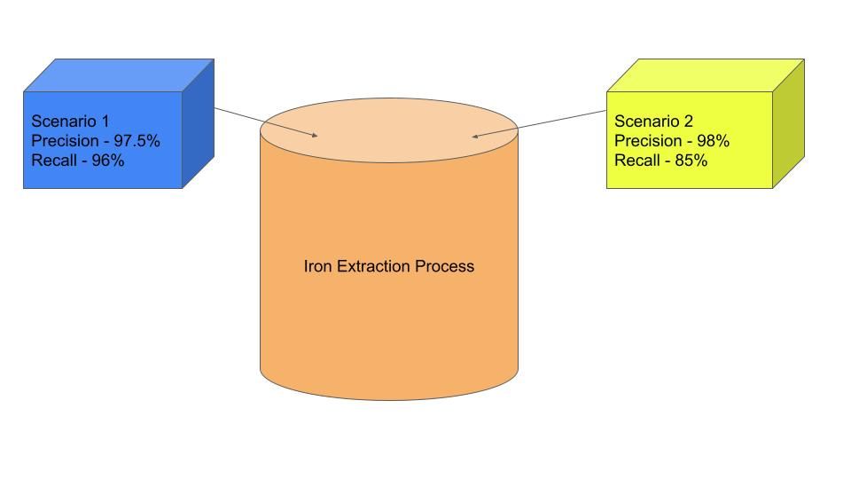
Illustration created by Author

Let’s say you follow the second method because you want purer iron from the furnace, which in turn means more waste in the process of extraction. Let’s assume if you increase the purity of iron by 0.5% to 98%, your waste of metal increases by 11%. That means the recall value corresponding to a precision value of 98% becomes 85%. This barter of the recall in exchange for higher precision and vice versa shows the inverse relation of precision and recall.

Wouldn’t it be great if you could know all the values of precision and corresponding values of recall so that you can make a decision that best suits your objective?

The precision-recall curve helps make that choice, and you will understand that in depth in the following sections. But before we do that, let's first understand an important concept of the threshold which is core to the PR curve. 

The Concept of Threshold

Let's pick an example of fraudulent transaction identification to understand how a threshold (or cutoff) works. The below table has four transactions with transaction IDs ranging from 1 to 4; a transaction can be either fraudulent or regular. The fraud detection model outputs the probability of a transaction being fraudulent (highlighted in the yellow column), which intrinsically gives away the probability of a regular transaction. 

A transaction is said to be predicted as fraudulent if the output probability is greater than the chosen threshold in the Probability of Fraud transaction column, else it is declared as a regular transaction. 

When a threshold which is as stringent as 0.9 is applied, the first three transactions are marked as regular, whereas the last transaction is marked as a fraudulent transaction. Such a high threshold exudes confidence in predictions leading to a high precision scenario. In return, you are sacrificing the model recall by missing out on some fraudulent transactions.

Such a scenario is not desirable despite high Precision. Can you think of why?

It is because the business ends up paying a higher cost of missing out on fraud identification which is the sole purpose of building such a model. Note that the cost of a fraudulent transaction is much higher than the cost involved in blocked but regular transactions, i.e., FP. 

Now, consider the other side of the spectrum with a low threshold value of 0.4 that marks the bottom three transactions as fraudulent. Such a liberal threshold will block the majority of the transactions, which can annoy many customers. Not to forget the additional burden on human resources to work through the flagged transactions and identify the true frauds.

Thus the business has to define target metrics and their desired values to get the best of both worlds, keeping the following costs under consideration:

• The cost of identifying a fraudulent transaction as regular (False Negatives)
• The cost of identifying a regular transaction as fraudulent (False Positive)

Referring back to the definition of precision, you would find that false positives is in the denominator of the mathematical expression which means minimizing false positives would maximize the precision. In the same way, minimizing false negatives would maximize the recall of the model.

Thus, whether a transaction is predicted as fraudulent or regular depends largely on the threshold value.

What is a Precision-Recall Curve?

A precision-recall curve helps you decide a threshold on the basis of the desirable values of precision and recall. It also comes in handy to compare different model performance by computing “Area Under the Precision-Recall Curve,” abbreviated as AUC.

As explained through the confusion matrix, a binary classification model will yield TP, FP, TN, and FN for various values of threshold, where each value of threshold outputs corresponding pair of precision and recall values. 

Plotting recall values on the x-axis and corresponding precision values on the y-axis generates a PR curve that illustrates a negative slope function. It represents the trade-off between precision (reducing FPs) and recall (reducing FNs) for a given model. Considering the inverse relationship between precision and recall, the curve is generally non-linear, implying that increasing one metric decreases the other, but the decrease might not be proportional.

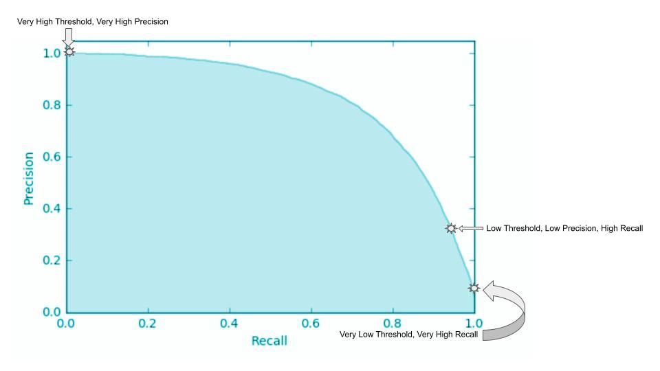
Image from StackExchange

Let’s say an organization chooses a minimum acceptable recall value of 98%. The precision stands at 30% at a crossover point represented by the star labeled “Low Threshold, Low Precision, High Recall.”  

The other two extreme points represent the cases where the threshold is:

• Too low leads to high Recall – the cost of human capital and annoyed customers
• Too high leads to high Precision – the cost of fraudulent transactions and loss of reputation.

Using a PR curve

In addition to deciding the right cut-off aligned with the business metric, the area under the curve of precision-recall curves from multiple models or algorithms can be used to compare their performance. It is particularly useful to compare models using PR curves rather than using individual precision, recall, or even an F1 score metric (which is a harmonic mean of Precision and Recall).

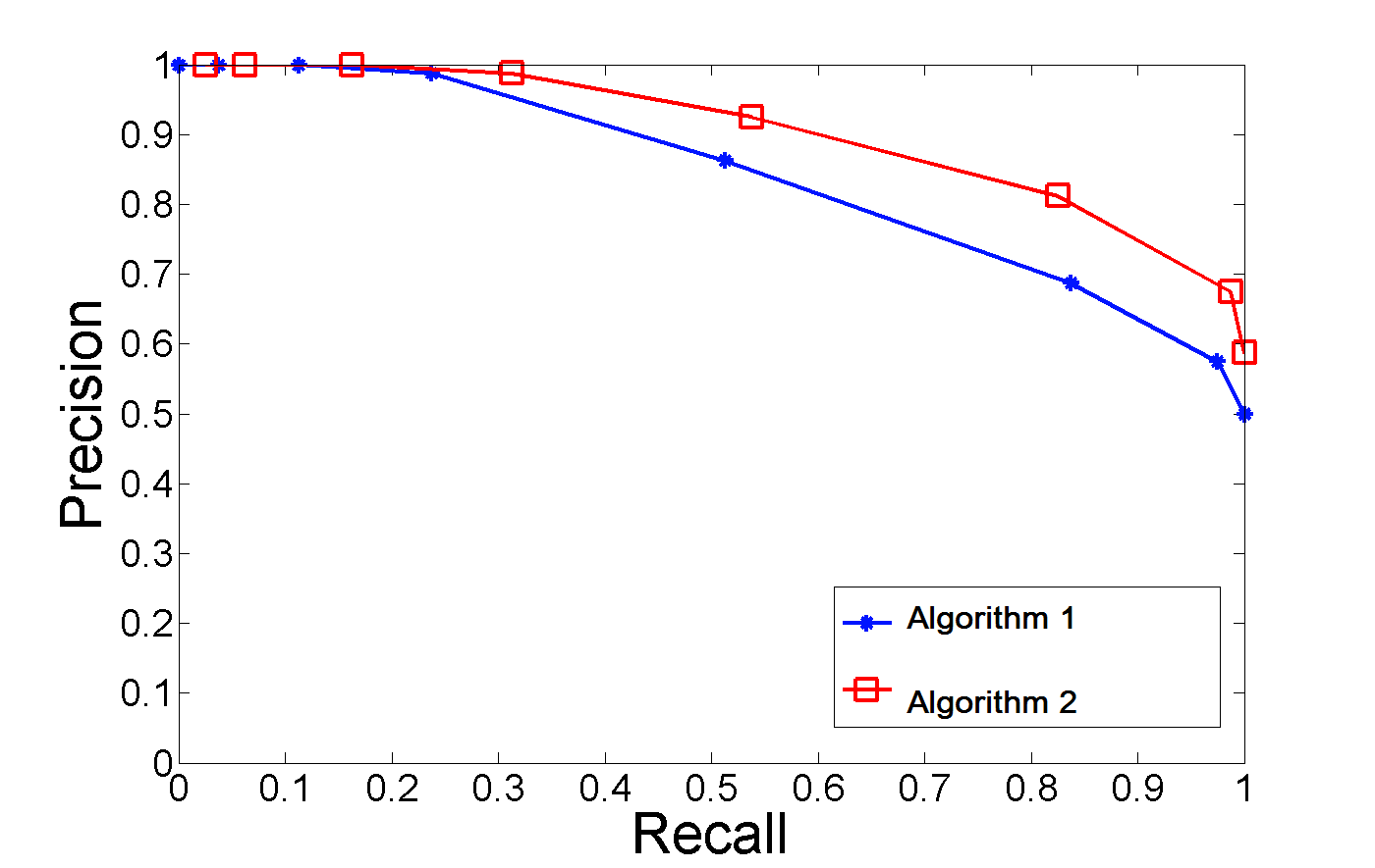
Image from Stackoverflow

Such metrics are threshold-dependent, wherein a change in threshold changes the distribution of TP, FP, and FN. Two different models can perform differently for a given threshold which makes the PR curve a robust choice for model comparison. The above plot illustrates two PR curves from two different algorithms on a given dataset – the AUC from algorithm two is greater than the AUC from algorithm one, making it a better choice for the given problem.

Implementing Precision-Recall Curve in Python

Now that we know what precision-recall curves are and what they’re used for, let’s look at creating a precision-recall curve in Python. 

Step 1: Import necessary Python packages

Let’s look at the model data set for breast cancer detection where “class 1” represents cancer diagnosis and “class 0” represents there is no cancer.

The first import loads the dataset from “sklearn.datasets” which includes the independent and the target variables. As it is a model dataset that can be easily learned by most algorithms, we have chosen the Naive Bayes algorithm imported as “GaussianNB” from sklearn. 

Next import of “Precision_Recall_curve” outputs different thresholds and their corresponding Precision and Recall values.

from sklearn.datasets import load_breast_cancer
from sklearn.naive_bayes import GaussianNB
from sklearn.metrics import precision_recall_curve
from sklearn.model_selection import train_test_split
import matplotlib.pyplot as plt

Step 2: Preparing train and test data

The independent variables are stored in the key “data” and the target variable in the key “target” within the “data” dictionary. The data is then split into the train and test sets by passing test_size argument with a value 0.3.

# Load model breast cancer data
data = load_breast_cancer()
X = data['data']
y = data['target']

Let’s have a look at the distribution of positive and negative class i.e. breast cancer and not a breast cancer cases.

import numpy as np
unique, counts = np.unique(y, return_counts=True)
plt.pie(counts, labels=unique, autopct='%.0f%%');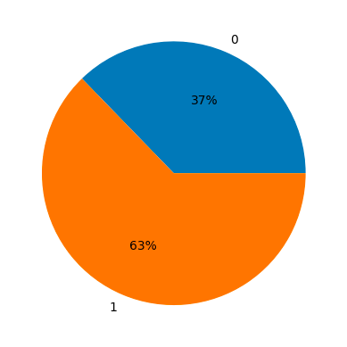

Split the data into train and test set using the train_test_split method from sklearn’s model_selection module.

X_train, X_test, y_train, y_test = train_test_split(X, y, test_size=0.3, random_state=0)

Step 3: Model Training

Training data is parsed as arguments to GaussianNB() to initiate the model training. The fitted model object is then used to get the predictions in the form of probability on the train and the test dataset. 

# Fit a Naive Bayes model
clf = GaussianNB().fit(X_train, y_train)

Step 4: Generating Predictions

Generate prediction probabilities using training and testing dataset which would be used to get Precision and Recall at different values of the threshold.

# Predict probability
y_prob_train = clf.predict_proba(X_train)[:,1]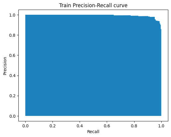
y_prob_test = clf.predict_proba(X_test)[:,1]

Step 5: Plotting PR curve

The Precision_Recall_curve() method takes two inputs – the probabilities from train dataset i.e. y_prob_train and the actual ground truth values, and returns three values namely Precision, Recall, and thresholds.

precision, recall, thresholds = precision_recall_curve(y_train, y_prob_train)
plt.fill_between(recall, precision)
plt.ylabel("Precision")
plt.xlabel("Recall")
plt.title("Train Precision-Recall curve");

The precision and recall vectors are used to plot the PR curve at varying thresholds as shown below:

PR Curve generated by Author

Is a Precision-Recall Curve Better Than a ROC Curve?

A ROC curve is similar to the PR curve but plots the True Positive Rate (TPR) vs the False Positive Rate (FPR) for different thresholds. We already know TPR, it is just another name for recall. So, let us focus on FPR, which signifies the number of misclassifications from the negative class. Continuing with the fraud example, it represents the percentage of regular transactions marked as fraudulent.

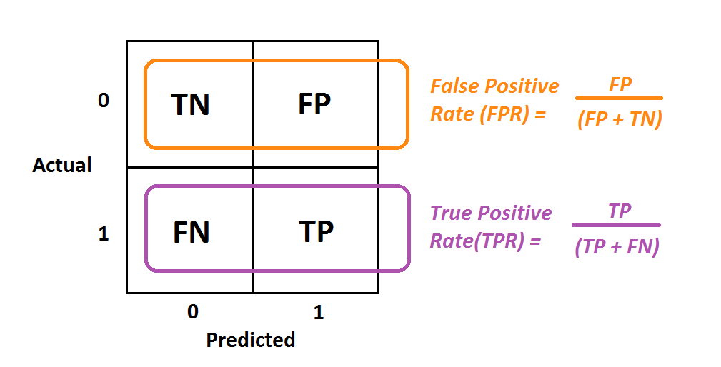
Image by Albert Um

By now, we understand that the recall, aka TPR, is common between the PR curve and ROC curve; the prime difference is that of precision and FPR respectively. Let’s see why a PR curve is more informative comparatively.

This is because the P-R curve provides more meaningful insights about the class of interest as compared to the ROC curve. Let’s pick the fraud transaction prediction. True Negatives (TN) in imbalanced dataset cases tend to be very large, making FPR a very tiny value. But does that say anything about the model’s performance in predicting a transaction as fraudulent?

No! On the other hand, using Precision as one of the metrics describes the model’s performance on the positive class (fraud transactions). This describes if the model is conservative vs liberal in marking fraudulent transactions.

The second major drawback of the ROC curve is its immunity to imbalanced data. From the figure above, you can see that FPR is a negative class-only metric, meaning that the change in FP is expected to be proportional to the change in FP+TN (all negative instances). Thus if the distribution of the underlying data changes, the ROC doesn’t change significantly. This insensitivity to class distribution makes the PR curve a better bet over the ROC curve.

Final Thoughts

Precision and recall are key evaluation metrics to measure the performance of machine learning classification models. However, the trade-off between the two depends on the business prerogative and is best resolved through the PR curve. The article explained how to interpret the PR curve and choose the right threshold to meet the business objective. Furthermore, the post illustrated a step-by-step tutorial on how to plot it using Python. We also discussed why the PR curve is more informative than the ROC curve.