course
Introduction to Data Visualization with Seaborn
4 hours
122K
Data visualization is a critical component in the interpretation of complex datasets.
In the realm of Python programming, Seaborn stands out as a powerful library for creating visually appealing and informative statistical graphics like histograms and line plots.
It builds on Matplotlib's capabilities, enhancing its interface and offering more options for visualizing data, especially for statistical analysis. Seaborn's seamless integration with Pandas DataFrames makes it a favorite among data scientists and analysts.
In this detailed guide, we will focus on one of the most commonly used plots in Seaborn—the histogram.
sns.histplot functionThe sns.histplot function in Seaborn is designed for drawing histograms, which are essential for examining the distribution of continuous data. This function is versatile and allows for extensive customization, making it easier to draw meaningful insights from the data.
This function is one of the many available functions from the Seaborn library. Have a look at this cheat sheet below for a quick overview.
Seaborn for data science cheat sheet - source
Before diving into data visualization, we need to set up our environment. This involves importing necessary libraries, with Seaborn being the primary focus. Seaborn is typically imported as sns for convenience.
Alongside Seaborn, other essential libraries often include NumPy for numerical operations, pandas for data handling, and Matplotlib for additional customization options.
import seaborn as sns
import pandas as pd
import numpy as np
import matplotlib.pyplot as plt
These are all essential libraries that provide the necessary tools for creating and manipulating data visualizations in Python. They are the most commonly used libraries for data analysts and data scientists.
If you’re getting started with learning Python, I suggest you try out our Introduction to Python course. For further learning on pandas, NumPy, and Matplotlib, our Data Manipulation with pandas, Introduction to NumPy, and Introduction to Data Visualization with Matplotlib courses.
We'll use the Boston Housing Prices dataset, which can be loaded from the Scikit-Learn library. This dataset provides housing values in different areas of Boston along with several attributes like crime rate, average number of rooms, etc.
from sklearn.datasets import load_boston
boston = load_boston()
df = pd.DataFrame(boston.data, columns=boston.feature_names)
df['MEDV'] = boston.target
Having suitable data for your histograms is what makes or breaks them. In this case, we are using a continuous variable, the median value of owner-occupied homes (MEDV) in Boston.
As histograms typically show the distribution of a single variable, we'll select one column from our DataFrame.
New to Scikit-Learn? Have a go at our tutorial on Python Machine Learning. If you’d like more information, our Supervised Learning with scikit-learn course will help cover the basics.
Before you start things out, here are some basic pre-requisites before you start building your Seaborn histogram:
We'll start by going through some of the common syntax and parameters of the `sns.histplot` function.
The basic syntax for creating a histogram using `sns.histplot` is straightforward.
Key parameters include:
data: The data set, which is often a Pandas DataFrame.x: The variable for which the histogram is plotted.color: To specify the color of the bars.alpha: Transparency of the bars.bins: The number of bins (bar groups) to be used.binwidth: The width of each bin.kde: A boolean to add a Kernel Density Estimate plot.hue: To differentiate data subsets based on another variable.The function accepts many parameters and arguments, but we'll focus on the ones needed for our dataset.
Let's create a basic histogram to visualize the distribution of median housing prices (MEDV).
plt.figure(figsize=(10, 6))
sns.histplot(data=df, x='MEDV')
plt.title('Distribution of Median Housing Prices in Boston')
plt.xlabel('Median Value of Owner-Occupied Homes (in $1000)')
plt.ylabel('Frequency')
plt.grid(True)
plt.show()
This command will display the histogram for the MEDV column.
Here's the generated plot from this code:
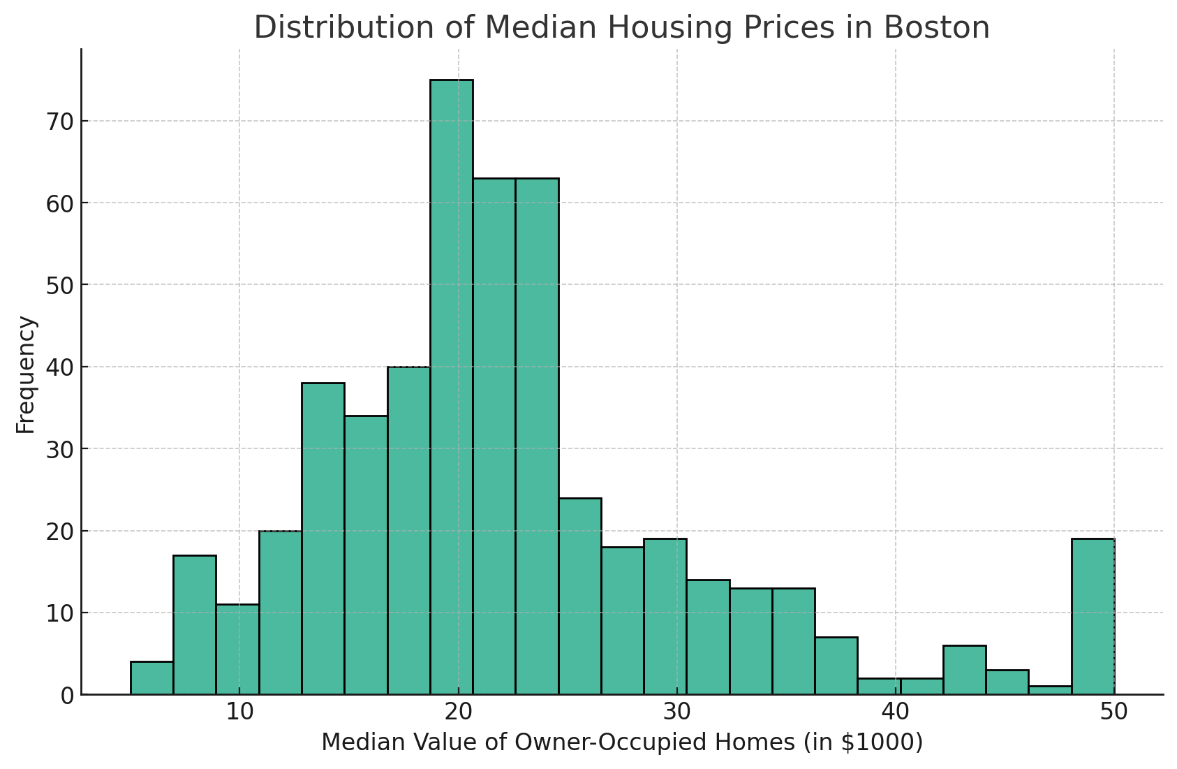
Here is the histogram plot showing the distribution of median housing prices (MEDV) in the Boston dataset. The histogram provides a visual representation of the frequency distribution of median values of owner-occupied homes.
Adjusting the number of bins can help in better understanding the distribution. A higher number of bins can reveal more details, whereas a lower number simplifies the visualization.
To increase the number of bins, you can modify the bins parameter.
Here's an example:
plt.figure(figsize=(10, 6))
sns.histplot(data=df, x='MEDV', bins=30)
plt.title('Distribution of Median Housing Prices in Boston')
plt.xlabel('Median Value of Owner-Occupied Homes (in $1000)')
plt.ylabel('Frequency')
plt.grid(True)
plt.show()
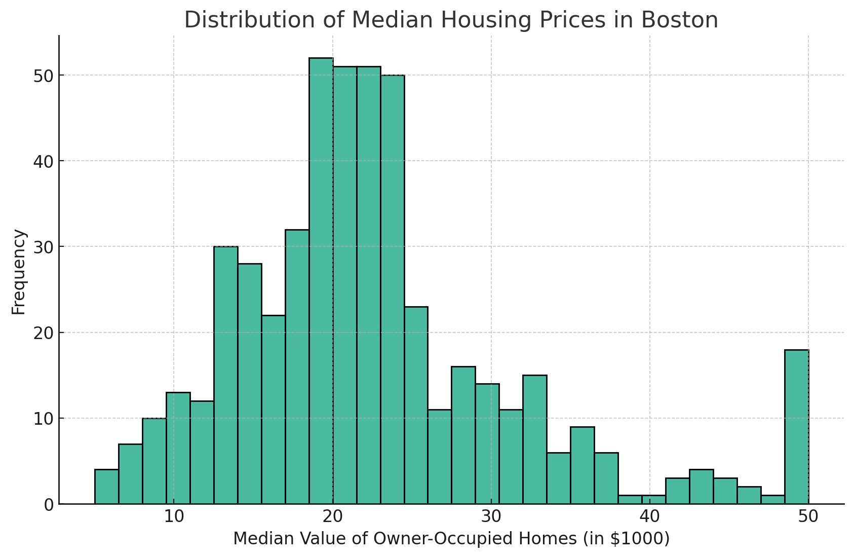
As you can see from the Seaborn histogram above, the number of bars has increased to the amount I have set, which, in this case, is 30. This is a good way to drill down into the details for more granularity of your data.
Customizing the aesthetics, like changing the bar color and transparency, can make the histogram more informative and visually appealing.
In the example below, I recreated our original histogram using purple instead of the default color.
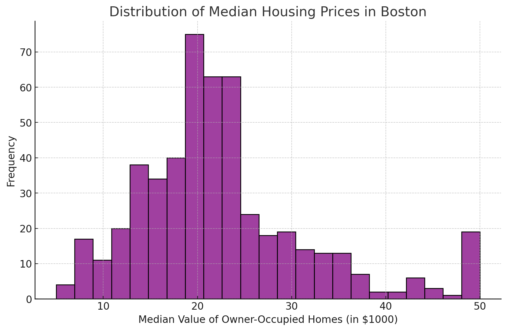
Here’s the code I used to create the chart above.
plt.figure(figsize=(10, 6))
sns.histplot(data=df, x='MEDV', color='purple')
plt.title('Distribution of Median Housing Prices in Boston')
plt.xlabel('Median Value of Owner-Occupied Homes (in $1000)')
plt.ylabel('Frequency')
plt.grid(True)
plt.show()
KDE provides a smooth estimate of the data distribution. It can be particularly useful for identifying patterns in the data.
This creates a smooth line curve that can help visualize the overall trends.
To achieve this, we then use kde parameter in this function:
plt.figure(figsize=(10, 6))
sns.histplot(data=df, x='MEDV', kde=True)
plt.title('Distribution of Median Housing Prices in Boston')
plt.xlabel('Median Value of Owner-Occupied Homes (in $1000)')
plt.ylabel('Frequency')
plt.grid(True)
plt.show()
This will produce a nice curve to our histogram, as shown below.
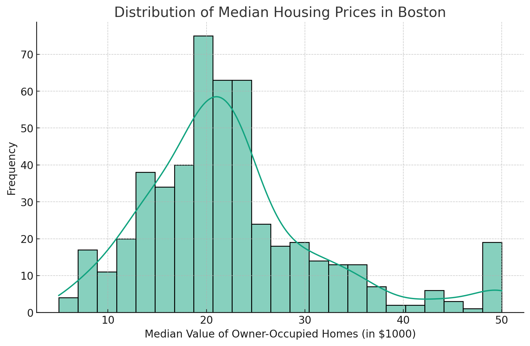
The addition of the Kernel Density Estimate (KDE) line gives a smoother estimate of the distribution.
The hue parameter allows for the comparison of different categories within the histogram.
This parameter allows us to distinguish between different categories within the same histogram, providing a visual comparison of distributions.
Simply put, it takes a categorical column from the DataFrame and differentiates the data using different colors.
For example, if we have a column named 'CHAS' in our DataFrame, which indicates whether a house is along the Charles River (1) or not (0), we can use the 'hue' parameter to compare the distribution of median housing prices for houses that are near the river versus those that aren't.
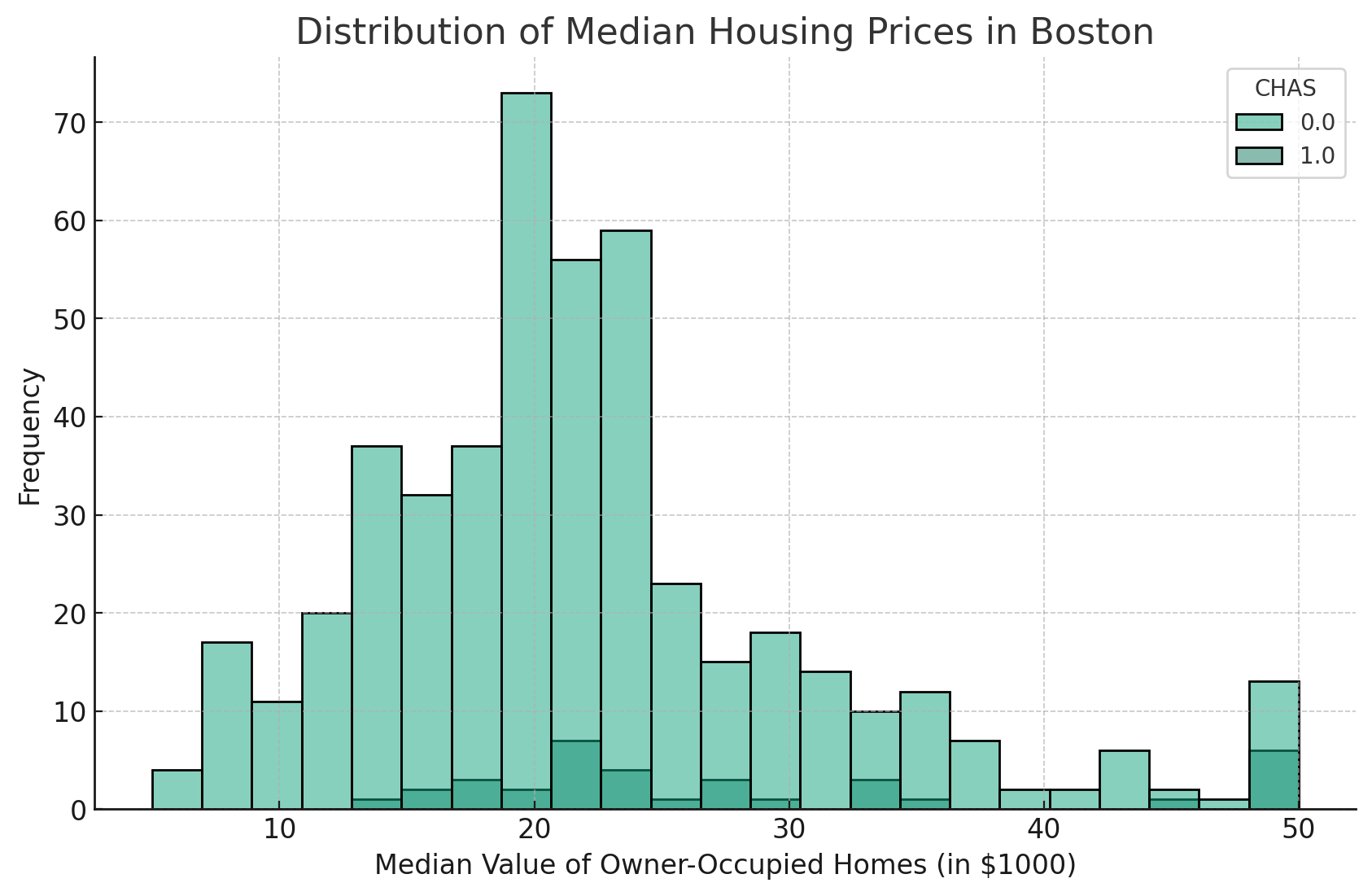
The code will look as follows:
plt.figure(figsize=(10, 6))
sns.histplot(data=df, x='MEDV', hue='CHAS')
plt.title('Distribution of Median Housing Prices in Boston')
plt.xlabel('Median Value of Owner-Occupied Homes (in $1000)')
plt.ylabel('Frequency')
plt.grid(True)
plt.show()
This will generate a histogram where the distribution of MEDV for homes bordering Charles River (CHAS=1) is differentiated from those not bordering the river (CHAS=0), each represented by a different color.
When you’re building Seaborn histograms, there are several aspects to bear in mind, as outlined below:
Selecting the optimal number of bins is key to creating an informative histogram. While a higher number of bins can provide more detail, it can also lead to overfitting and misrepresenting the data.
On the other hand, too few bins may oversimplify the distribution.
One way to choose the right number of bins is by using a rule of thumb called Scott's Rule. This rule calculates the ideal bin size based on the number of data points in the dataset.
While it is important to provide enough detail in a histogram, ensuring that the visualization remains clear and easy to interpret is also crucial.
Adding too many elements, like KDE lines or too many colors, can lead to cluttered visuals that are difficult to understand.
It's best to strike a balance between adding informative elements and maintaining simplicity.
The type of data being visualized also plays a role in selecting the appropriate histogram parameters.
For example, continuous variables will require different bin sizes compared to categorical variables.
It's important to consider the nature of the data while creating histograms to ensure that they accurately represent the distribution.
However, Seaborn is just one of the libraries that are available out there for data visualization in Python. You can also consider creating your histograms in Matplotlib instead if you prefer.
Seaborn is a powerful library for creating visualizations in Python, and the `histplot` function allows for the easy creation of histograms. Just by changing the parameters within the function, you’re able to modify how your chart looks to achieve the level of detail and aesthetics that you want.
Do remember all the Seaborn histogram tips mentioned above: always consider the type of data, choose appropriate bin sizes, and balance detail with clarity when creating histograms using Seaborn.
Interested in learning more about Seaborn and its other powerful data visualization capabilities? Our Introduction to Data Visualization with Seaborn course is an excellent course for beginners.
Start Your Seaborn Journey Today!
course
course
course
cheat sheet
Karlijn Willems
2 min
tutorial
Joleen Bothma
9 min
tutorial
Elena Kosourova
12 min
tutorial
Kurtis Pykes
12 min
tutorial
Moez Ali
20 min
tutorial
Aditya Sharma
8 min